RDF Triple Stores vs. Labeled Property Graphs: What’s the Difference?

Editor’s Note: This presentation was given by Jesús Barrasa at GraphConnect San Francisco in October 2016.

Presentation Summary

Resource Description Framework (RDF) triple stores and labeled property graphs both provide ways to explore and graphically depict connected data. But the two are very different – and each have different strengths in different use cases.

In this presentation, Dr. Jesús Barrasa starts with a brief history of both RDF triple stores and the labeled property graph model, including the origins of the Semantic Web.

Then, he breaks down the major data model differences between RDF and a labeled property graph, including the rich internal structure of a labeled property graph (absent in RDF), and the differences in size, with RDFs being an order of magnitude bigger than a labeled property graph in many cases.

Next, Barrasa details several small but important differences between RDF and labeled property graphs. To accommodate some of these distinctions, he presents three RDF workarounds to mimic the same qualities of a labeled property graph.

Going further, Barrasa compares both the graph query languages and data store architecture of both graph technologies.

In conclusion, Barrasa takes a closer look at semantics within an RDF triple store and then concludes with a brief demo of all of the discussed differences.

Full Presentation: How Semantic Is Your Graph?

What we’re going to be talking about today are two types of graphs: the RDF graph and the property graph that implements Neo4j:

A Brief History: The RDF and Labeled Property Graph

Let’s go over a brief history on where these two models come from. RDF stands for Resource Description Framework and it’s a W3C standard for data exchange in the Web. It’s an exchange model that represents data as a graph, which is the main point in common with the Neo4j property graph.

It understands the world in terms of connected entities, and it became very popular at the beginning of the century with the article the Semantic Web published in Scientific American by Tim Berners-Lee, Jim Hendler and Ora Lassila. They described their vision of the Internet, where people would publish data in a structured format with well-defined semantics in a way that agents — software — would be able to consume and do clever things with.

Next, persisting RDF — storing it — became a thing, and these stores were called triple stores. Next they were called quad stores and included information about context and named graphs, then RDF stores, and most recently they call themselves “semantic graph database.”

So what do they mean by the name “semantic graph database,” and how does it relate to Neo4j?

The labeled property graph, on the other hand, was developed more or less at the same time by a group of Swedish engineers. They were developing a ECM system in which they decided to model and store data as a graph.

The motivation was not so much about exchanging or publishing data; they were more interested in efficient storage that would allow for fast querying and fast traversals across connected data. They liked this way of representing data in a way that’s close to our logical model — the way we draw a domain on the whiteboard.

Ultimately, they thought this had value outside the ECM they were developing and a few years later their work became Neo4j.

The RDF and Labeled Property Graph Models

Now, taking into account the origin of both things — the RDF model is more about data exchange and the labeled property graph is purely about storage and querying — let’s take a look at the two models they implement. By now you all know that a graph is formed of two components: vertices and the edges that connect them. So how do these two appear in both models?

In a labeled property graph, vertices are called nodes, which have a uniquely identifiable ID and a set of key-value pairs, or properties, that characterize them. In the same way, edges, or connections between nodes – which we call relationships — have an ID. It’s important that we can identify them uniquely, and they also have a type and a set of key value of pairs — or properties that characterize the connections.



The important thing to remember here is that both the nodes and relationships have an internal structure, which differentiates this model from the RDF model. By internal structure I mean this set of key-value pairs that describe them.

On the other hand, in the RDF model, vertices can be two things. At the core of RDF is this notion of a triple, which is a statement composed of three elements that represent two vertices connected by an edge. It’s called subject-predicate-object. Subject will be a resource, or a node in the graph. The predicate will represent an edge – a relationship — and the object will be another node or a literal value. But here, from the point of view of the graph, that’s going to be another vertex:



The interesting thing to know is that resources (vertices/nodes) and relationships (edges) are identified by a URI, which is a unique identifier. This means that neither nodes nor edges have an internal structure; they are purely a unique label. That’s one of the main differences between RDF and labeled property graphs.

Let’s take a look at an example to make this a bit more clear:



Here’s a rich snippets that Google returns when you do a search for Sketches of Spain, which is one of my favorite albums by Miles Davis. This search returns a description of the album with things like the artist, the release date, the genre, producers and some awards. I’m going to represent this information in both models below.

Below is one of the possible serializations of RDF called Turtle syntax:



You can see that the triples are identified by a URI, which is the subject. The predicate is the name and the object will be Sketches of Spain, which together is a sequence of triples. So these are the kinds of things you will have to write if you want to insert data in a triple store.

Let’s look at how this information is displayed graphically:



The nodes on the left represent the album, which has a set of edges coming out of it. The rectangles represent literal values — the description: album about Miles Davis, the genre, the title — and it has connections to other things that are in ellipses that represent other resources (i.e., other nodes in the graph) that have their own properties and attributes.

What this means is that by representing data in RDF with triples, we’re kind of breaking it down to the maximum. We’re doing a complete atomic decomposition of our data, and we end up finding nodes in the graph that are resources and also literal values.

Now let’s look at it from the point of view of the labeled property graph. What I’ve created below is a sequence of Cypher statements that contain exactly the same information as the Turtle syntax above:



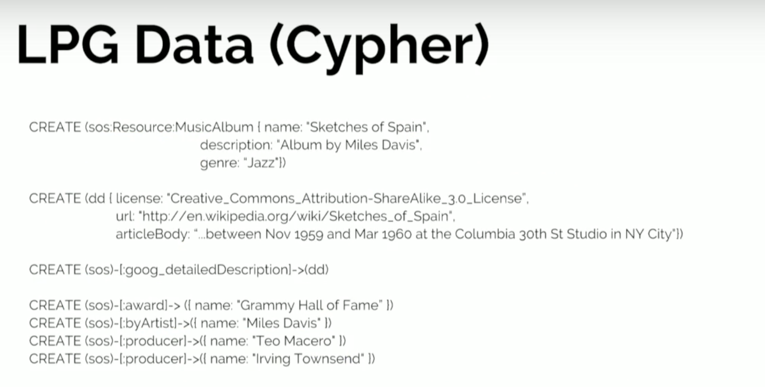
The semantics are the same. There’s no standard serialization format, or a way of expressing a labeled property graph, but rather a sequence of CREATE statements do the job here.

We create a node, which is more obviously represented with a parenthesis, and then the attributes — or the internal structure — in the curly bracket: the name, the description and the genre. Likewise, the connections between nodes are described with hard brackets.

Below is what the labeled property graph looks like:



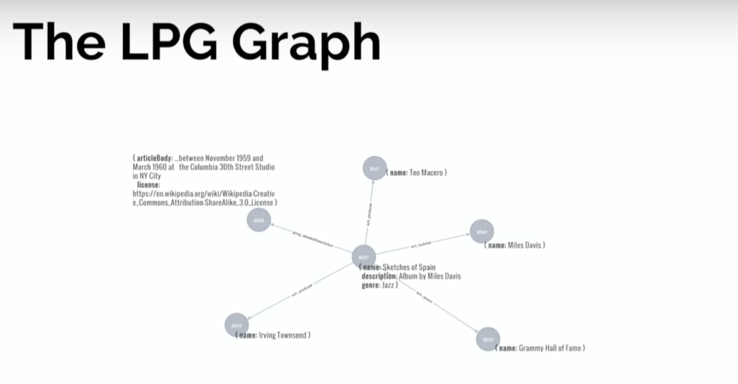
The first impression is that it’s much more compact. Even though it has certain elements in common with the RDF graph, it’s completely different because nodes have this internal structure and values of attributes don’t represent vertices in the graph.

This allows for a much more reduced structure. But we still have the album at the center, which is connected to a number of entities, but the title, name and description aren’t represented by separate nodes. That’s a first distinction.

Sometimes there’s confusion when we compare the two models. If you have a graph with two billion triples, how do the two compare in terms of nodes, for example? If we take a graph with n nodes with five properties per node, five attributes, five relationships and five connections, we would get 11 triples per node in a labeled property graph.

Again, I’m not comparing storage capacity, but keep in mind that when you have a 100 million triple graph (i.e., RDF graph), that’s an order of magnitude bigger than a labeled property graph. That same data will probably be equivalent to a ten-million-node labeled property graph.

Key Differences Between RDF and Property Graphs

Difference #1: RDF Does Not Uniquely Identify Instances of Relationships of the Same Type

Now that we know a bit more about the two models, let’s compare differences in terms of exclusivity.

The first one is quite important, and that is the fact that in RDF it’s not possible to uniquely identify instances of a relationship. In other words, we can say: it’s not possible to have connections of the same type between the same pair of nodes because that would represent exactly the same triple, with no extra information.

Let’s look at the following as an example, a labeled property graph and an RDF graph in which Dan cannot like Ann three times; he can only do it once:



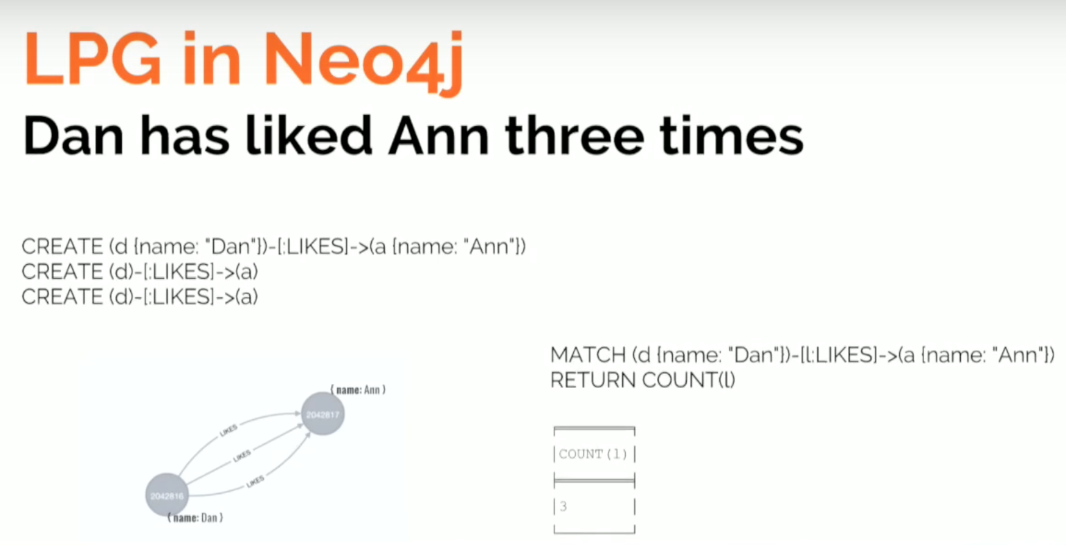
We create a node called Dan that LIKES Anne. I repeat that Dan likes Anne two more times, and I end up with a graph that has three connections of type LIKES between Dan and Ann. Good.

Not only can we visualize this in a helpful way, but we can also query it to ask, “How many times does this pattern appear in the graph?” which returns a count of three.

Now let’s try to do the same in RDF using SPARQL:



What insert a statement that says Dan has name Dan, Ann has name Ann and Dan LIKES Ann, which we repeat three times. But see the graph that we get instead (above).

We have the values of the properties as vertices of the graph, and we have Dan with name Dan. We have Ann with name Ann, and we have a single connection between them, which is sad, because Dan liked her three times.

If I do the count again searching for this particular triple pattern, and I do the count, I get one. The reason for that is it’s not possible to identify unique instances of relationships of the same type with an RDF triple store.

Difference #2: Inability to Qualify Instances of Relationships

Second, because you can’t identify these unique instances in RDF, you cannot qualify them or give them attributes. Let’s take a look at another example that explores flights between New York City and San Francisco:



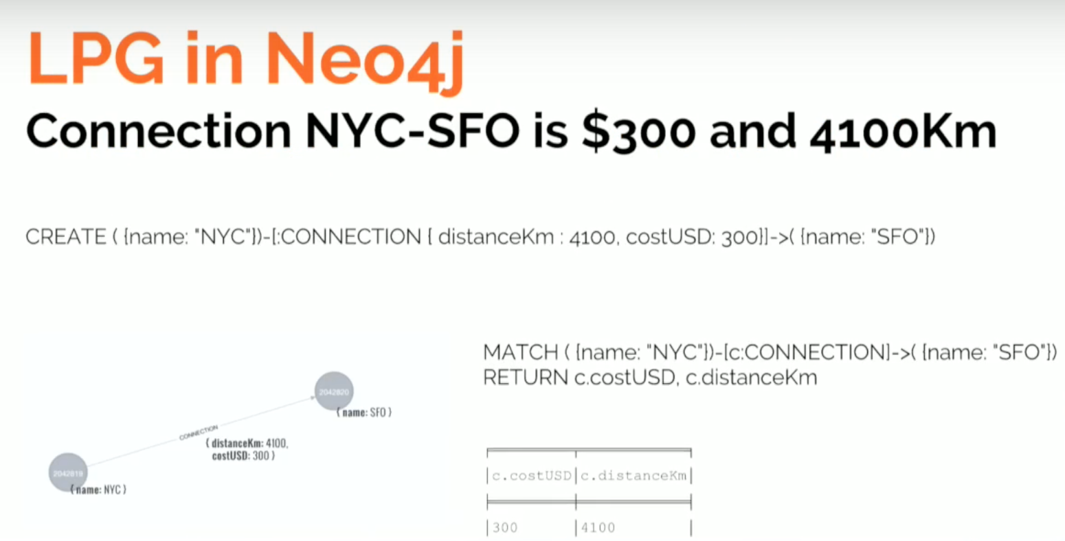
It costs $300 and is a total of 4,100 kilometers. Again, this statement can be expressed in Neo4j’s graph query language, Cypher, saying that there’s a connection between New York City and San Francisco, and that the connection has two attributes: the distance and the cost in dollars.

We produce a nice graph and can query the cost and distance of the connection to return two nodes.

If I try to do the same in RDF, I encounter a problem:



In this query, we say there’s a city called New York, a city called San Francisco, and a connection between them.

But how do I state the fact that this connection has a cost? I could try to say something like, “Connection has a distance.” But which connection? That would be a global property of the connection, so you can’t express that in RDF. As you can see above, here’s the graph that this type of SPARQL query produces.

RDF Workarounds

There are a few alternatives for these weaknesses in RDF.

One of them is a data modeling workaround, but we’re going to see that this is the same problem we experience with a relational models. What happens when we have these many-to-many relationships — people knowing people, and people being known by others? This provides an entity-relationship model, but then you have to translate this into tables with several JOINs.

Because the modeling paradigm doesn’t offer you a way to modeling these types of relationships, you have to use what you have on hand and represent it the way you can. And as you know, the problem is that this starts building a gap between your model as you conceive it, and the model that you store and query. There are two alternate technical approaches to this problem: reification and singleton property.

Below is one RDF data modeling workaround, which is the simple option:



Because in RDF we don’t have attributes in relationships, we create an intermediate node. On the left is what I can do in the labeled property graph. Because we can’t create such a simple model in RDF, we create an entity that represents the connection between New York and San Francisco.

Once I have that node, I can get properties out of it. This alternative isn’t too bad; the query will be more complicated, but okay.

Now let’s take a look at reification, which — as you can see — isn’t very readable:



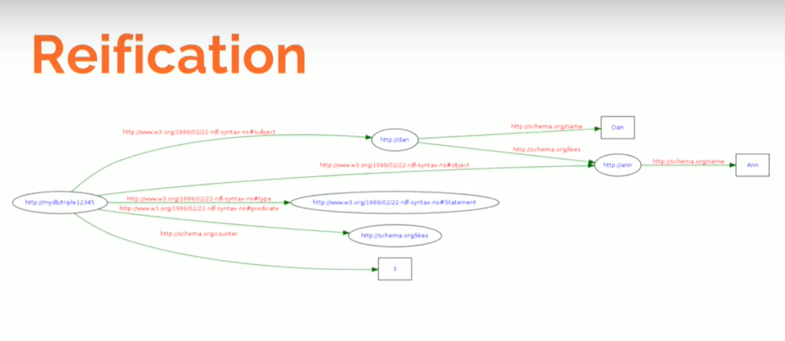
We still have Dan with with name Dan, and Ann with name Ann with a connection saying that he likes her.

With reification, we create a metagraph on top of our graph that represents the statement that we have here. We create a new node that represents a statement and points at the subject Dan, at the object Ann, and at the property stating the fact that he likes her. Now that I have an object — a node — I can add a counter, which tells us three.

This is quite ugly. On the one hand, you can still query who Ann likes:



But if you want to query “how many times,” you have to go look at both the graph and the metagraph. So if Dan likes Ann, then look at the statement that connects Dan and Ann and get the counter.

Now, imagine if you need to update that. You would have to say, “Dan has liked her one more time.” You wouldn’t come and say, “Add one more” because that doesn’t add more information. You will have to come and say, “Grab a pattern, take the value in the counter, increase it by one, and then set the new value.”

The Singleton property is another modeling alternative pretty much in the same vein:



You have your original model — Dan with his name who likes Ann, with her name. You can give this relationship a unique name, ID1234, which allows us to describe it. We can say it’s an instance of likes and I can give it a counter of three.

Again, I’m building a metamodel that — while more compact than the reification model — still doesn’t allow you to ask, “Who does Dan like?” You have to ask, “Who does Dan 1234?” which is the type like.

Difference #3: RDF Can Have Multivalued Properties and the Labeled Property Graph Can Have Arrays

In RDF you can have multi-value properties — triples where the subject and predicate are the same but the object is different — which is fine. In the labeled property graph you have to use arrays, which is the equivalent.



In the snippet we had before, we had an album that had two values for the genre property: jazz and orchestral jazz. That’s easy to express in triples, and in Cypher you will need to use an array — not too bad.

Difference #4: RDF Uses Quads for Named Graph Definition

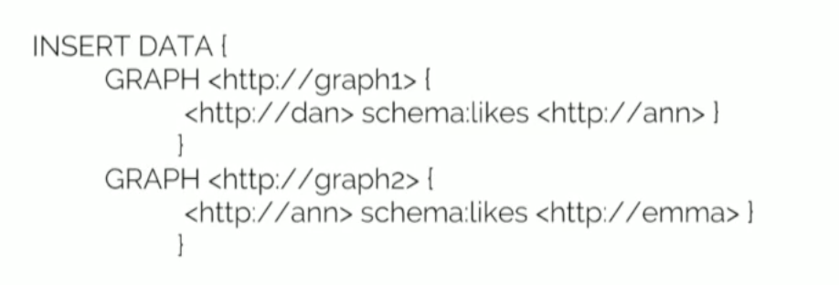
Another difference is this notion of quad, which has no equivalent in labeled property graphs. You can add context or extra values to triples that identifies them and makes it easy to define subgraphs, or named properties.

We can state that Dan likes Ann in graph one and Ann likes Emma in another graph:

RDF & Labeled Property Graph Query Languages

The two different models also rely on different database query languages.

Because of the atomic decomposition of the data and RDF, you typically have longer patterns when you perform queries. Below is a query that has the names of artists with albums produced by Irving Thompson:



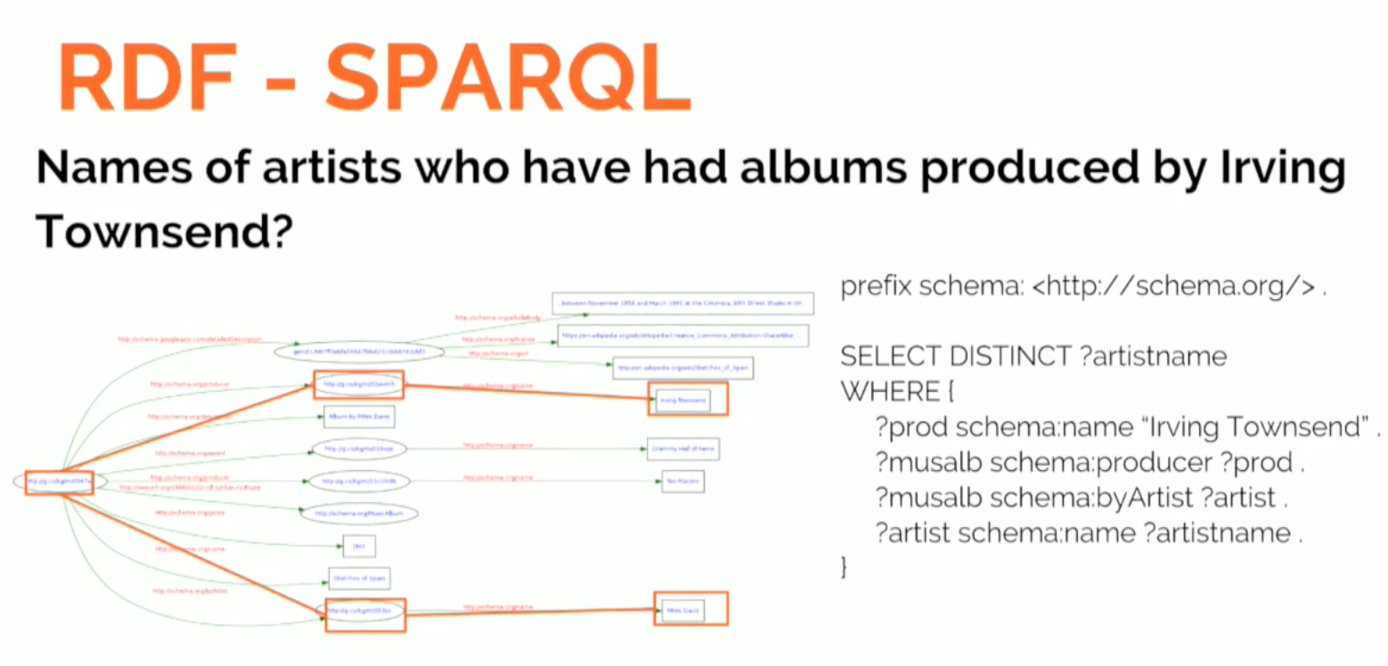
You have four patterns, each of which represents each of the edges in the more compact labeled property graph. But this isn’t what I would call an essential differentiator.

There were a few recent updates to both the SPARQL and Cypher query languages:



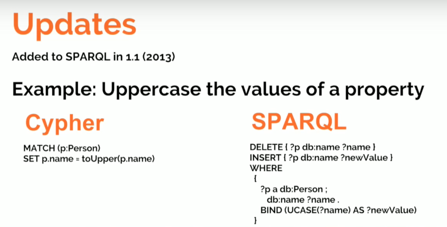
Something like uppercasing the values of a property in Cypher is very SQL-like and simple.

You can much a person and attribute name to uppercase, whereas in SPARQL you will have to MATCH it, BIND it to a variable, do the uppercase, and then do the insertion and the deletion because we can have multiple values. So by updating you need to delete the previous value, unless you want to keep both of them.

RDF & Labeled Property Graph Data Stores

RDF stores are very strongly index-based, while Neo4j is navigational. It implements index-free adjacency, which means that it stores the connections between connected entities, between connected nodes, in disks.

This means that when you query Neo4j, you’re actually chasing pointers instead of scanning indexes. We know that index-based storage is okay for queries that aren’t very deep, but it’s very difficult to do something like path analysis. Compare that to Neo4j, which allows you to have native graph storage that is best for deep or variable-length traversals and path queries.

It’s fair to say that triple stores were never meant to be used in operational and transactional use cases. They should be used in mostly additive, typically slow-changing — if not immutable — datasets. For example, the capital of Spain is Madrid, which isn’t likely to change. Conversely, Neo4j excels in highly dynamic scenarios and transactional use cases where data integrity is key.

A Comparison: Semantics

So what do we mean when we say semantics?



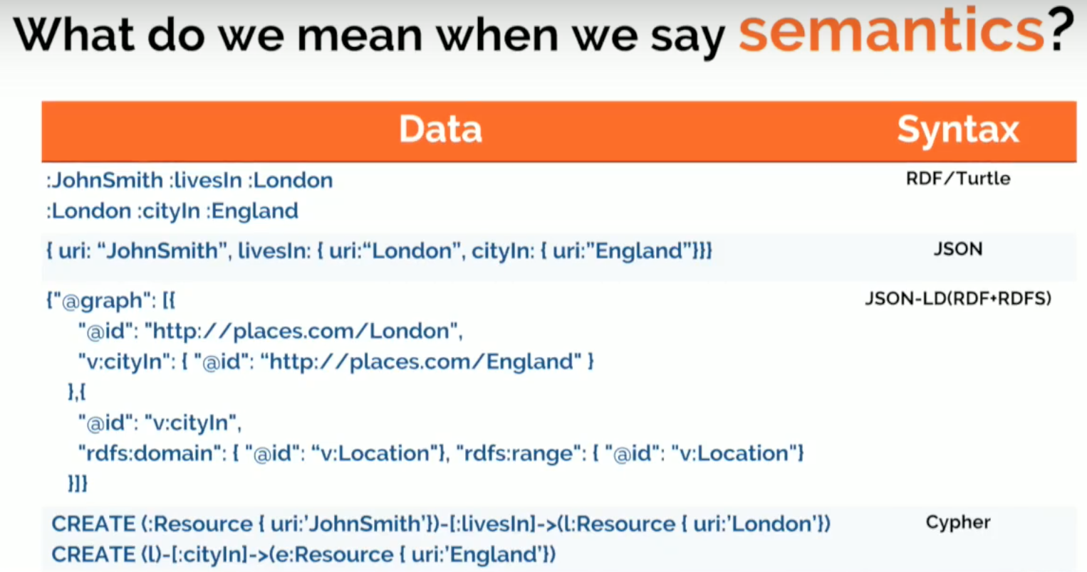
The first two lines are on the front end of RDF in total notation, saying that John Smith lives in London and that London is a city in England. The second one is a fragment of JSON that could easily represent the same information. The third one is JSON-LD and includes both the data and the ontology, and the final one is a fragment of Cypher.

Semantics can mean two things in the RDF world. The first is the idea of vocabulary-based semantics. Because you can identify relationships with URIs, you can define agreed-upon vocabularies like Schema.org and Google Knowledge Graph (GKG). This covers most of the usage of RDF today.

The other meaning is inference-based semantics, which is rule-based — including OWL. We use this when we want to express what the data means so that I can infer facts, do some reasoning or check the consistency of the dataset.

Let’s look at a couple examples. The first example provides a simple pair of facts: John lives in London. London is in England. You can express this with two RDF triples:

:JohnSmith :livesIn :London
:London :locationIn :England

Now you run a query: who lives in England? You can express that in SPARQL:

SELECT ?who
WHERE { ?who :livesIn :England }

But it returns zero results because you have to say:

?x :livesIn ?city ^
?city :cityIn ?ctry
=> ?x :LivesIn ?ctry

If someone lives in a city and the city is in a country, then you live in the country. But no one’s going to figure that out if you don’t make it explicit in a rule, and this is an example of how you have to make the semantic explicit. The real question is: are your semantics explicit?

If we ask the question again, now that we have defined our rule, it will return John Smith.

Below is another example that shows importing data from two data sources into a triple store. There are two facts coming from datasource1: Jane Smith’s email is jsmith@gmail.com, and her Twitter handle is @jsmith. This can look like the following two triples:

:JaneS1 :hasEmail 'jsmith@gmail.com'
:JaneS1 :hasTwitterHandle '@jsmith'

Now we get another pair of triples from another data source that says: Jane Smith’s email is jsmith@gmail.com and her LinkedIn profile is “https://linkdn.com/js.” Again, the two triples below look like this:

:js2 :hasEmail 'jsmith@gmail.com'
:js2 :hasLnkdnProfile 'https://linkdn.com/js'

Next you put it into the RDF graph thinking that semantics are going to do the magic. You ask the question: What’s the LinkedIn profile of the person tweeting as @jsmith? The SPARQL query looks like this:

SELECT ?profile
WHERE {  []  :hasTwitterHandle '@jsmith' ; :hasLnkdnProfile ?profile . }

But again you get no results, because — like in the previous case — you have to say that the email address is a unique identifier and therefore you can infer that if two resources have the same email, you can derive that they’re the same and can be expressed with a rule like this one:

 
?x :hasEmail ?email ^
?y :hasEmail ?email
=> ?x owl:sameAs ?y

You can also express this more elegantly in OWL, which would look like this:

:hasEmail rdf:type
owl:InverseFunctionalProperty
 
?prop a owl:InverseFunctionalProperty ?p^
?x ?p ?al
=> owl:sameAs ?y

An inverse functional property is a primary-key-style property. It’s not exactly the same because a primary key is a kind of constraint that would prevent you from adding data to your database if there’s another one with the same value.

Here, you can add data without any problem. But if we find two that have the same value, we’re going to think that these two are the same.

Even if we express this in a more declarative way, these are the semantics of an inverse functional property. Basically if two values have the same value, I can derive that they are the same. We re-run the query and this time it will return Jane Smith’s LinkedIn profile.

It’s all about making the data explicit. There’s really no magic here; RDF is just a way of making data more intelligent and making your semantics explicit. Below is a quote from Tim Burners-Lee that speaks to this:

A Demo: How Do We Get to a Semantic Graph Database?

I’m going to show features and capabilities in Neo4j that are typically from RDF as stored procedures and extensions. Hopefully, they’ll make their way into the APOC library soon.



So what are the takeaways from this demo? The first one was mentioned in the presentation by the Financial Times, an organization that made the transition from RDF to a labeled property graph.

They thought they needed a linked semantic data platform to connect their data, but what they actually needed was a graph. So always ask yourself what kind of features you need. Is it about the inferencing? Is it about semantics? Or is it just a graph?

If you store your data in RDF and query it in SPARQL, you’re not semantic — you have a graph. In most of the use cases, you find yourself not using as much of OWL and all the semantic capabilities as you would, because you know it’s extremely complex and it results in performance issues. If you’re working with a reasonably-sized dataset, don’t expect it to finish the query.

We also know that publishing RDF out of Neo4j is trivial, which is the same with importing RDF. The code is under 100 lines and is available on Github. It’s a really simple task.

And I’ve also shown that inference doesn’t require OWL. In the end, semantics (inference) is just data-driven, server-side logic, typically implemented as rules. You’re putting some intelligence close to your data that’s in turn driven by an ontology. And if you manage to balance expressivity and performance without falling into unneeded complexity, then it may be a useful tool.

I’m not going to criticize OWL because its own creators discuss why it’s not being adopted. It’s definitely not taking off, and I think one of the reasons is because it can be overkill for many use cases.