Using Neo4j to Take Us to the Stars

Software Engineer, AllThingsGraphed.com
10 min read

Editor’s Note: Last October at GraphConnect San Francisco, Caleb Jones – Software Engineer and Blogger at AllThingsGraphed.com – delivered this presentation on how to route interstellar voyages using Neo4j.
For more videos from GraphConnect SF and to register for GraphConnect Europe, check out graphconnect.com..
I’m going to start with the history of computing and how it’s catapulted us into the current graph world we live in. I’ll also showcase a variety of graphs — some of which are also on my blog — that are network analysis visualizations.
Organized Complexity and the History of Computing
The scientist Warren Weaver wrote an essay in 1948 called Science and Complexity in which he broke down the history of science into three epochs. The first epoch deals with the problem of simplicity.
Take, for example, Newtonian mechanics in which you have one object acting on another object. But we know that no system is that simplistic; it’s more likely that you have one object that acts on multiple other objects. When you scale this up into the millions and billions, the model suddenly breaks down.
The next scientific period — during which he wrote his essay — dealt with the problem of disorganized complexity, during which people understood many of the elements operating in a system but only at a system level. In other words, people were studying a system attribute that was itself disconnected from the notion of elements acting on each other.
Weaver predicted the next epoch having the problem of organized complexity in which you understand both that many elements operate in a system and also understand the system taking those interactions and elements into account. That, to me, just screams graph because within graphs we have attributes that include relationships.
What I find most interesting is that he predicted that addressing organized complexity would require computational power far beyond what they had available in 1948. The phone you have in your pocket is far more powerful than any conceivable computer that they had at that time.
This level of computational power is what has propelled us into our current world of graphs; Neo4j couldn’t do what it does without this computational power.
Consider the following chart that shows memory over time (note that the y axis is logarithmic):

The cost of computing and storage trail each other by about five or ten years, and you can see that a lot of these projects — such as Neo4j and Hadoop — were birthed as a result of our hardware being liberated. Spark, which is memory-based, came along about six years later as the cost of memory decreased. Transistor cost and internet transit cost also plummeted. All together, these changes culminated into a world of computational power.
Graphs Are Everywhere!
What is your passion? Is it your work, music, books? Whatever your passion, is there a way to graph it?
To demonstrate that, below are a series of visualizations I did on my blog AllThingsGraphed. On the left is my LinkedIn network, and on my right is my Facebook network:

Below is a network of interactions of proteins in budding yeast, which comes from an open dataset that I downloaded:

And what is a protein? It’s a molecule, which is itself is a graph because it’s compiled of atoms connected to other atoms, each of which have different attributes:

Below is an open dataset of U.S. airline connections, which you can export into Google Earth and then fly through your graph, which is kind of fun:

We can make graphs out of other open datasets such as word definitions, comic books, acting careers on IMDB and more.
Graphing the Stars
It was my fascination with space at an early age that led me to the conclusion that we can ask big questions and use tools to get meaningful answers. And this is exactly what we are doing with graphs: We’re able to ask bigger questions because now we have the tools to answer them.
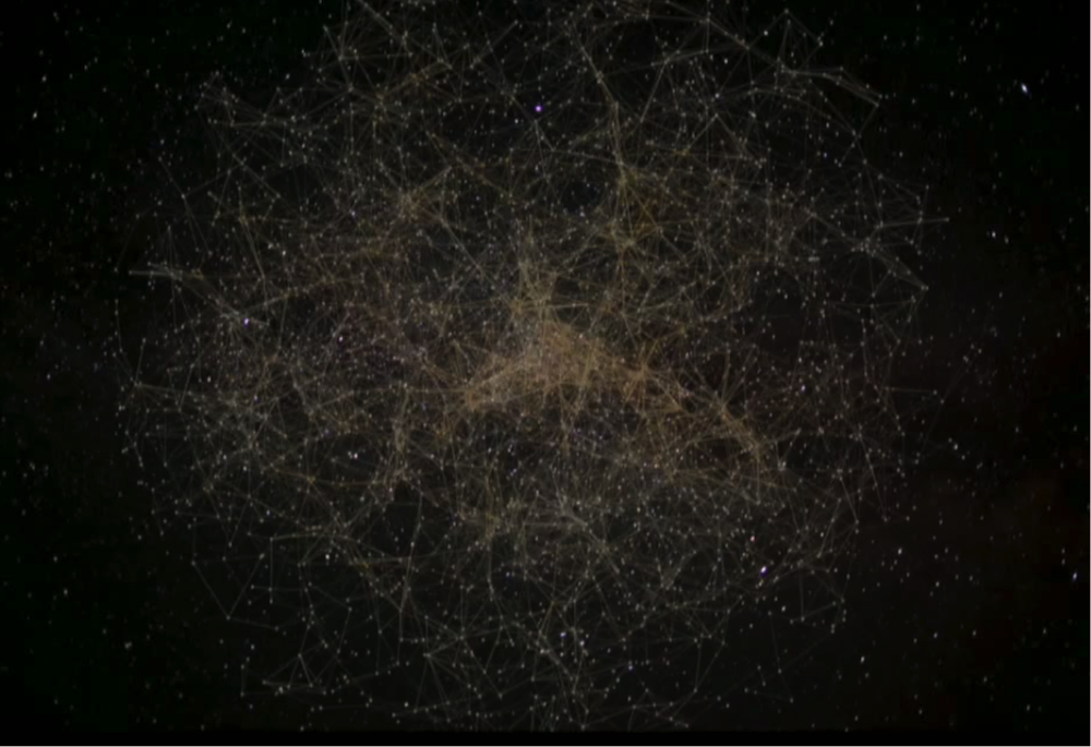
Below is a set of constellations:

If you look at these in this context, you can see that constellations really are three-dimensional graphs; they are composed of a series of connected nodes on a dome that is projected around us.
Take a look at the below video clip to watch a three-dimensional exploration of the constellations:
And below is a time-lapsed image of a SpaceX launch:

With space exploration, we are starting to build edges out to things beyond earth. We’re forging these networks in which every launch is an edge and every destination is a node. This allows us to ask some big questions, such as:
- How far would we have to be able to travel for our stellar neighborhood to open up?
- What would the navigational pathways of the stellar travel look like?
As we seek to answer these questions, we have to bring along the underlying assumptions:
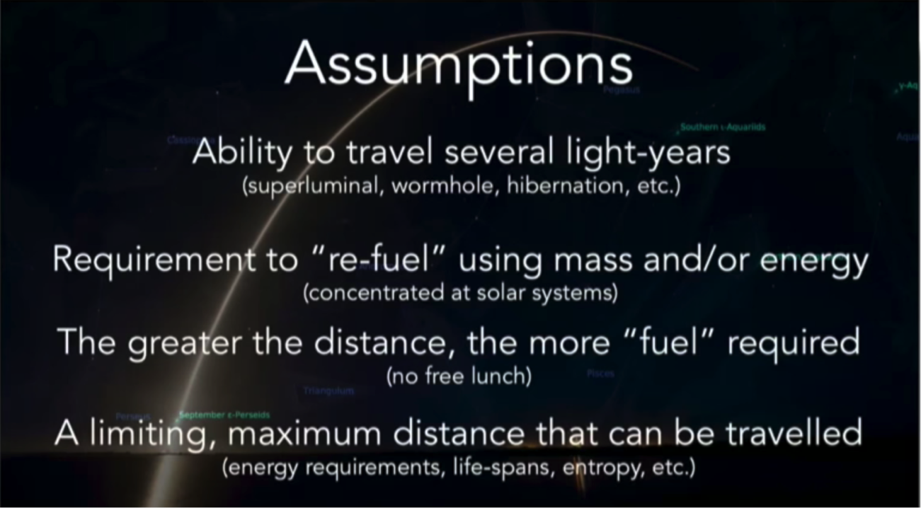
Neo4j and Space Travel
Now we can ask the question: How far would we have to travel in order for our stellar neighborhood to open up?
The first thing we need to do is calculate the distance from earth to all the other stars in this dataset, which is a range of five to 75 light years. Next we need to find the maximum distance that fully connects the stars.
This brings us to the concept of network components. On one extreme you have a graph with no edges, while on the other extreme you have a graph in which every node is perfectly connected.
But you can also have a graph in the spectrum in which you can get from one node to another but through a very indirect path. If you have a graph like that, it has a single connected component. So, to find out how far we’d need to travel to reach all of these stars, you could load all the nodes — the stars — up in a network and figure out if there’s one component.
Below is a graph that shows components per max light year:

If we can only travel five light years (before re-fueling, etc.), we have about 1400 isolated pockets of which we are just one. We can only reach maybe one or two others of our closest neighboring star systems.
If we bump it up to six light years we have significantly fewer at 1088. And if we keep moving up in light years we arrive at 14, which leaves us with a graph with a single connected component. This shows that if we really want to travel everywhere in our immediate stellar neighborhood, we need to travel in the range of nine to 14 light years.
One thing to note is that this network is basically a sphere with lots of interesting inter-fillamental structures, but on the outside of the sphere this stops. It doesn’t mean there’s nothing beyond that sphere, it’s just how far our dataset went. Regardless, the nine to 14 range seems to narrow this down, and we’re starting to get a little bit of sharpness to the answer of our question.
We can also ask the inverse question: How many stars are reachable, depending on how far we can travel? We know that the further we can travel the more connected we are, and the further we can travel the more stars we can reach.

What’s really fascinating about this is the flat line there. If we only travel five to seven light years, we are stuck in our own neighborhood. But as soon as we pass eight light years, we end up in a much more accessible neighborhood.
With the previous charts, we are able to answer our initial question, how far would we have to travel in order for our stellar neighborhood to open up? A reasonable answer is 12 light years, plus or minus a couple of light years. With the power of networks and graphs, we answered a question that may have initially seemed totally rhetorical. And this brings us back even further to graphing your passion.
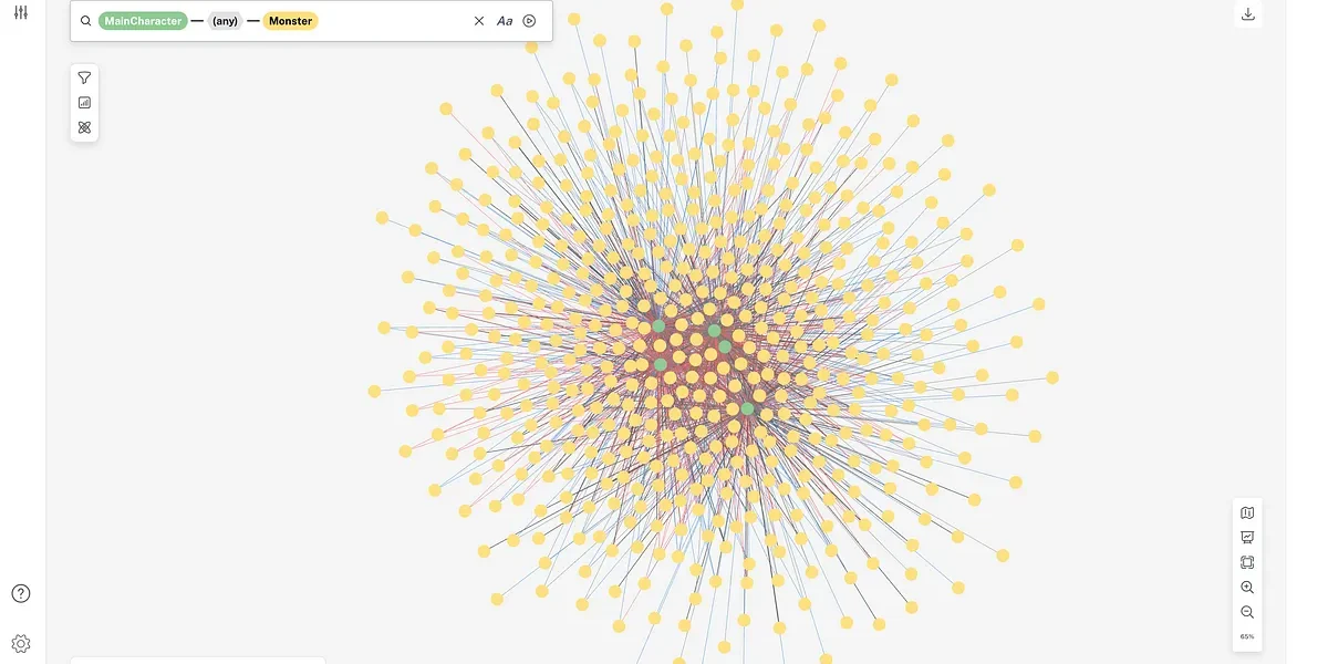
Let’s explore a new question: What would the navigational pathways of that travel look like? Earlier we were looking at line charts; now let’s look at our network:
This network is heliocentric, so our sun is right there in the center. Eventually we will want to look at this in a 3D graph but even in its 2D state, we can see a little bit of structure — a filamental arc, etc. Are there any hubs in our star network? We can answer this question by using betweenness centrality.
If you have a network you also have pathways, particularly if you have a network with a single component in which you will have a pathway — whether direct or indirect — from any one node to any other node. Betweenness centrality calculates every possible path and each time you calculate that path you increment the counter on that node. If we size the nodes based on their centrality score, we end up with the following:
I added some color to the nodes using the using the Harvard spectral classification which is based on the temperature of the stars. We are the bluish-white dot at the center; we’re not the smallest, but we’re also not the largest.
But why stellar hubs? Why is this the interesting question or important question?
Because if we were to identify common traveling routes, we would also want to set up intuitive waypoints or stations. And where you travel is where you develop major cities and civilizations. If I put on my Search for Extraterrestrial Intelligence (SETI) hat, I might ask: What if there are already stellar faring civilizations out there? Hubs like these might be an interesting place to look.
Interestingly, even in our heliocentric dataset, we didn’t receive a high centrality score. Below are the hubs in our stellar neighborhood:

Let’s ask another question: What would the navigational pathways of stellar travel look like? So far, we’ve been looking at our graphs in 2D, which hides a lot of features. To create a 3D graph, we can use a tool developed by the University of Toronto called NAViGaTOR.
Below is a visualization at seven light years:
At eight light years:
At nine light years:
And at 12 light years:
Below is a view looking out from the sun at the navigational pathways to other stars around it:
Michael Hunger’s Neo4j shell tools allow you to import this 3D network into Neo4j, after which you can run Dijkstra’s algorithm to return the shortest path.
Below is the code I wrote to find the shortest path:

There are a few parameters you need to figure out and describe how you want them to traverse your network. For example, you can use the Dijkstra’s algorithm to simply figure out the number of hops to determine degrees of separation. In this case, our paths are all based on distance so our algorithm needs to place a weight on the edge.
We want to find the shortest path between the sun and the star Vega. Our code returns the following JSON document, which essentially acts as interstellar directions:

These directions start from the sun and provides its coordinates (which are all 0, since it is at the center). To get to the next star, Gl-699, you have to travel 5.98 light years. From there you travel 9.4 light years to get to the next star, and so on and so forth. At the end, we have the number of hops it takes to get to Vega, as well as its total distance from the sun.
Another interesting thing to explore is the travel distance and hops for different max distances to Vega:

At eight light years your travel distance jumps up to about 55, and you’re going to have to make nine hops, which will kill your distance. If you move up to nine light years, you’ll have to make only six hops so you can save a little bit of distance. And we again see this same range that keeps coming up in this dataset — twelve plus or minus two — so it flat-lines.
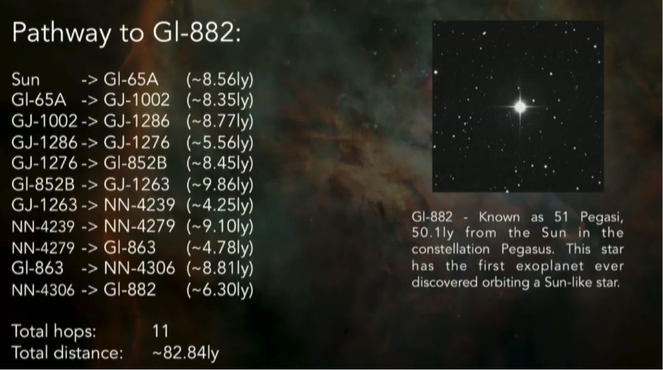
I found a few additional stars for which to run the Dijkstra’s algorithm in Neo4j. The first is 51 Pegasi, which is a the first star with a confirmed exoplanet:
Another one is GL667 which, at the time when I did this it had a confirmed exoplanet with the highest earth similarity index on it. A feature that’s notable on this one is that it’s a triple star system. That would be like a potentially habitable planet with three stars, and it’s only about three hops to get to once we have that network figured out:

Now that we’ve asked and answered all these questions — what’s next?

These are just a few of the items that I hope we can explore together in the coming years – stay tuned for more at AllThingsGraphed.com.
Inspired by Caleb’s talk? Register for GraphConnect Europe on April 26, 2016 at for more presentations, workshops and lightning talks on the evolving world of graph database technology.
Share Article


Explore
Related Articles
Bolster Your Cybersecurity by Visualizing Attack Graphs With Neo4j & G.V()


15 Best Graph Visualization Tools for Your Neo4j Graph Database