RDBMS & graphs: SQL vs. Cypher query languages


12 min read
When it comes to a database query language, linguistic efficiency matters.
Querying relational databases is easy with SQL. As a declarative query language, SQL allows both for easy ad hoc querying in a database tool as well as specifying use-case related queries in your code. Even object-relational mappers use SQL under the hood to talk to the database.
But SQL runs up against major performance challenges when it tries to navigate connected data. For data-relationship questions, a single query in SQL can be many lines longer than the same query in a graph database query language like Cypher (more on Cypher below).
Lengthy SQL queries not only take more time to run, but they are also more likely to include human coding mistakes because of their complexity. In addition, shorter queries increase the ease of understanding and maintenance across your team of developers.
For example, imagine if an outside developer had to pick through a complicated SQL query and try to figure out the intent of the original developer – trouble would certainly ensue.
But what level of efficiency gains are we talking about between SQL queries and graph queries? How much more efficient is one versus another?
The answer: Fast enough to make a significant difference to your organization.
The efficiency of graph queries means they run in real time, and in an economy that runs at the speed of a single tweet, that’s a bottom-line difference you can’t afford to ignore.
In this RDBMS & Graphs blog series, we’ll explore how relational databases compare to their graph counterparts, including data models, query languages, deployment paradigms and more. In previous weeks, we explored why RDBMS aren’t always enough, graph basics for the relational developer and relational vs. graph data modeling
This week, we’ll compare query languages for both relational and graph databases, specifically examining SQL (the de facto query language of RDBMS) and Cypher (the most widely used graph query language).
The critical relationship between query languages and data modeling
It’s worth noting that a query language isn’t just about asking (a.k.a. querying) the database for a particular set of results; it’s also about modeling that data in the first place.
We know from last week that data modeling for a graph database is as easy as connecting circles and lines on a whiteboard. What you sketch on the whiteboard is what you store in the database.
On its own, this ease of modeling has many business benefits, the most obvious of which is that you can understand what your database developers are actually creating. But there’s more to it: An intuitive model built with the right database query language ensures there’s no mismatch between how you built the data and how you analyze it.
A query language represents its model closely. That’s why SQL is all about tables and JOINs while Cypher is about relationships between entities. As much as the graph model is more natural to work with, so is Cypher as it borrows from the pictorial representation of circles connected with arrows which any stakeholder (whether technical or non-technical) can understand.
In a relational database, the data modeling process is so far abstracted from actual day-to-day SQL queries that there’s a major disparity between analysis and implementation. In other words, the process of building a relational database model isn’t fit for asking (and answering) questions efficiently from that same model.
Graph database models, on the other hand, not only communicate how your data is related, but they also help you clearly communicate the kinds of questions you want to ask of your data model. Graph models and graph queries are just two sides of the same coin.
The right database query language helps us traverse both sides.
An introduction to Cypher, the graph query language
Just like SQL is the standard query language for relational databases, Cypher is an open, multi-vendor query language for graph technologies. The advent of the openCypher project has expanded the reach of Cypher well beyond just Neo4j, its original sponsor.
Cypher – also a declarative query language – is built on the basic concepts and clauses of SQL but with added graph-specific functionality, making it simple to work with a rich graph model without being overly verbose.
(Note: This introduction isn’t a reference document for Cypher but merely a high-level overview.)
Cypher is designed to be easily read and understood by developers, database professionals and business stakeholders alike. It’s easy to use because it matches the way we intuitively describe graphs using diagrams.
If you have ever tried to write a SQL statement with a large number of JOINs, you know that you quickly lose sight of what the query actually does, due to all the technical noise. In contrast, Cypher syntax stays clean and focused on domain concepts since queries are expressed visually.
The basic notion of Cypher is that it allows you to ask the database to find data that matches a specific pattern. Colloquially, we might ask the database to “find things like this,” and the way we describe what “things like this” look like is to draw them using ASCII art.
Consider the social graph below describing three mutual friends:

A social graph describing the relationship between three friends.
If we want to express the pattern of this basic graph in Cypher, we would write:
(emil)<-[:KNOWS]-(jim)-[:KNOWS]->(ian)-[:KNOWS]->(emil)
This Cypher statement describes a path which forms a triangle that connects a node we call jim to the two nodes we call ian and emil, and which also connects the ian node to the emil node. As you can see, Cypher naturally follows the way we draw graphs on the whiteboard.
Now, while this Cypher pattern describes a simple graph structure it doesn’t yet refer to any particular data in a graph database. To bind the pattern to specific nodes and relationships in an existing dataset we first need to specify some property values and node labels that help locate the relevant elements in the dataset.
Here’s our more fleshed-out Cypher pattern:
(emil:Person {name:'Emil'})
     <-[:KNOWS]-(jim:Person {name:'Jim'})
     -[:KNOWS]->(ian:Person {name:'Ian'})
     -[:KNOWS]->(emil)
Here we’ve bound each node to its identifier using its name property and Person label. The emil identifier, for example, is bound to a node in the dataset with a label Person and a name property whose value is Emil. Anchoring parts of the pattern to real data in this way is normal Cypher practice.
The RDBMS developer’s guide to Cypher clauses
Like most query languages, Cypher is composed of clauses.
The simplest queries consist of a MATCH clause followed by a RETURN clause. Here’s an example of a Cypher query that uses these two clauses to find the mutual friends of a user named Jim (from our social graph pictured above):
MATCH (a:Person {name:'Jim'})-[:KNOWS]->(b:Person)-[:KNOWS]->(c:Person), (a)-[:KNOWS]->(c)
RETURN b, c
Let’s look at each clause in further detail:
MATCH
The MATCH clause is at the heart of most Cypher queries.
Using ASCII characters to represent nodes and relationships, we draw the data we’re interested in. We draw nodes with parentheses, just like in these examples from the query above:
(a:Person {name:'Jim'})
(b:Person)
(c:Person)
(a)
We draw relationships using using pairs of dashes with greater-than or less-than signs (--> and <--) where the < and > signs indicate relationship direction. Between the dashes, relationship names are enclosed by square brackets and prefixed by a colon, like in this example from the query above:
-[:KNOWS]->
Node labels are also prefixed by a colon. As you see in the first node of the query, Person is the applicable label.
(a:Person … )
Node (and relationship) property key-value pairs are then specified within curly braces, like in this example:
( … {name:'Jim'})
In our original example query, we’re looking for a node labeled Person with a name property whose value is Jim. The return value from this lookup is bound to the identifier a. This identifier allows us to refer to the node that represents Jim throughout the rest of the query.
It’s worth noting that this pattern:
(a)-[:KNOWS]->(b)-[:KNOWS]->(c), (a)-[:KNOWS]->(c)
could, in theory, occur many times throughout our graph, especially in a large user dataset.
To confine the query, we need to anchor some part of it to one or more places in the graph. In specifying that we’re looking for a node labeled Person whose name property value is Jim, we’ve bound the pattern to a specific node in the graph — the node representing Jim.
Cypher then matches the remainder of the pattern to the graph immediately surrounding this anchor point based on the provided information on relationships and neighboring nodes. As it does so, it discovers nodes to bind to the other identifiers. While a will always be anchored to Jim, b and c will be bound to a sequence of nodes as the query executes.
RETURN
This clause specifies which expressions, relationships and properties in the matched data should be returned to the client. In our example query, we’re interested in returning the nodes bound to the b and c identifiers.
Other Cypher clauses
Other clauses you can use in a Cypher query include:
WHERE
Provides criteria for filtering pattern matching results.
CREATE and CREATE UNIQUE
Creates nodes and relationships.
MERGE
Ensures that the supplied pattern exists in the graph, either by reusing existing nodes and relationships that match the supplied predicates, or by creating new nodes and relationships.
DELETE/REMOVE
Removes nodes, relationships and properties.
SET
Sets property values and labels.
ORDER BY
Sorts results as part of a RETURN.
SKIP LIMIT
Skip results at the top and limit the number of results.
FOREACH
Performs an updating action for each element in a list.
UNION
Merges results from two or more queries.
WITH
Chains subsequent query parts and forwards results from one to the next. Similar to piping commands in Unix.
If these clauses look familiar – especially if you’re an RDBMS developer – that’s great! Cypher is intended to be easy-to-learn for SQL veterans while also being simple enough for beginners. (Click here for the most up-to-date Cypher Refcard to take a deeper dive into the Cypher query language.)
SQL vs. Cypher query examples: The good, the bad and the ugly
Now that you have a basic understanding of Cypher, it’s time to compare it side by side with SQL to realize the linguistic efficiency of the former – and the inefficiency of the latter – when it comes to queries around connected data.
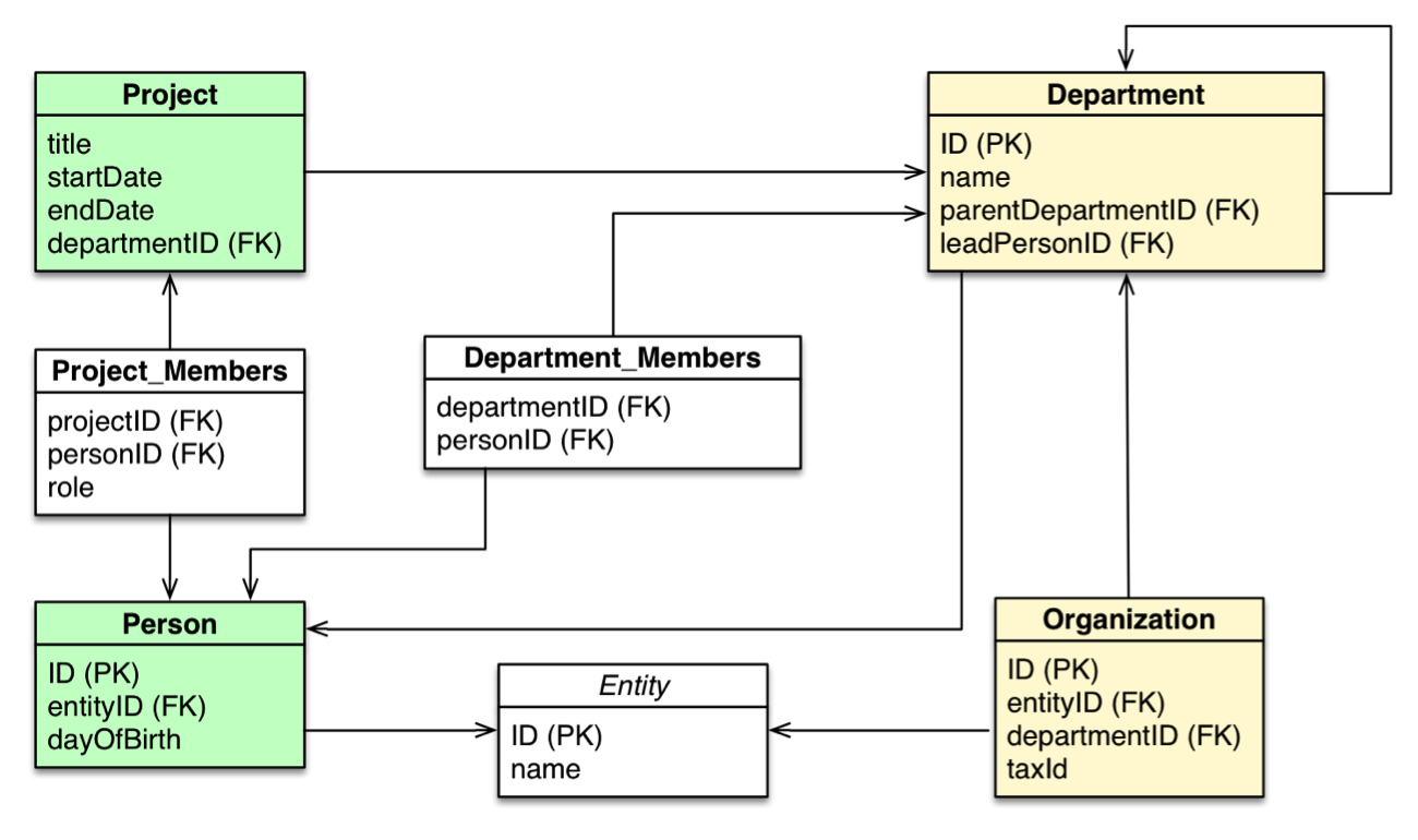
Our first example uses the organizational domain (from last week) pictured below as a relational data model:
A relational data model of an organizational domain.
In the organizational domain depicted in the model above, what would a SQL statement that lists the employees in the “IT Department” look like? And how does that statement compare to a Cypher statement?
SQL statement:
SELECT name FROM Person

LEFT JOIN Person_Department

  ON Person.Id = Person_Department.PersonId

LEFT JOIN Department

  ON Department.Id = Person_Department.DepartmentId

WHERE Department.name = "IT Department"
Cypher statement:
MATCH (p:Person)<-[:EMPLOYEE]-(d:Department)
WHERE d.name = "IT Department"
RETURN p.name
In this example on the previous page, the Cypher query is half the length of the SQL statement and significantly simpler. Not only would this Cypher query be faster to create and run, but it also reduces chances for error.
Now for another example, this one more extreme. We’ll start with the Cypher query:
Cypher statement:
MATCH (u:Customer {customer_id:'customer-one'})-[:BOUGHT]->(p:Product)<- [:BOUGHT]-(peer:Customer)-[:BOUGHT]->(reco:Product)
WHERE not (u)-[:BOUGHT]->(reco)
RETURN reco as Recommendation, count(*) as Frequency
ORDER BY Frequency DESC LIMIT 5;
This Cypher query says that for each customer who bought a product, look at the products that peer customers have purchased and add them as recommendations. The WHERE clause removes products that the customer has already purchased, since we don’t want to recommend something the customer already bought.
Each of the arrows in the MATCH clause of the Cypher query represents a relationship that would be modeled as a many-to-many JOIN table in a relational model with two JOINs each. So even this simple query encompasses potentially six JOINs across tables.
Here’s the equivalent query in SQL:
SQL statement:
SELECT product.product_name as Recommendation, count(1) as Frequency
FROM product, customer_product_mapping, (SELECT cpm3.product_id, cpm3.customer_id
FROM Customer_product_mapping cpm, Customer_product_mapping cpm2, Customer_product_mapping cpm3
WHERE cpm.customer_id = ‘customer-one’
and cpm.product_id = cpm2.product_id
and cpm2.customer_id != ‘customer-one’
and cpm3.customer_id = cpm2.customer_id
and cpm3.product_id not in (select distinct product_id
FROM Customer_product_mapping cpm
WHERE cpm.customer_id = ‘customer-one’)
) recommended_products
WHERE customer_product_mapping.product_id = product.product_id
and customer_product_mapping.product_id in recommended_products.product_id
and customer_product_mapping.customer_id = recommended_products.customer_id
GROUP BY product.product_name
ORDER BY Frequency desc
This SQL statement is three times as long as the equivalent Cypher query. It will not only suffer from performance issues due to the JOIN complexity but will also degrade in performance as the dataset grows.
Conclusion
When it comes to application performance, your database query language matters.
SQL is well-optimized for relational database models, but once it has to handle complex, relationship-oriented queries, its performance quickly degrades. In these instances, the root problem doesn’t lie with SQL but with the relational model itself, which isn’t designed to handle connected data.
For domains with highly connected data, the graph model is a must, and as a result, so is a graph query language like Cypher. If your development team comes from an SQL background, then Cypher will be easy to learn and even easier to execute.
When it comes to your next graph-powered, enterprise-level application, you’ll be glad that the query language underpinning it all is build for speed and efficiency.
Next week, we’ll explore different deployment paradigms for relational and graph databases, including polyglot persistence.
Want to learn more on how relational databases compare to their graph counterparts? Download this ebook, The Definitive Guide to Graph Databases for the RDBMS Developer, and discover when and how to use graphs in conjunction with your relational database.
Catch up with the rest of the RDBMS & Graphs series:
Share Article


Explore
Related Articles

Neo4j Named “One to Watch” in Snowflake’s 2026 Modern Marketing Data Stack Report
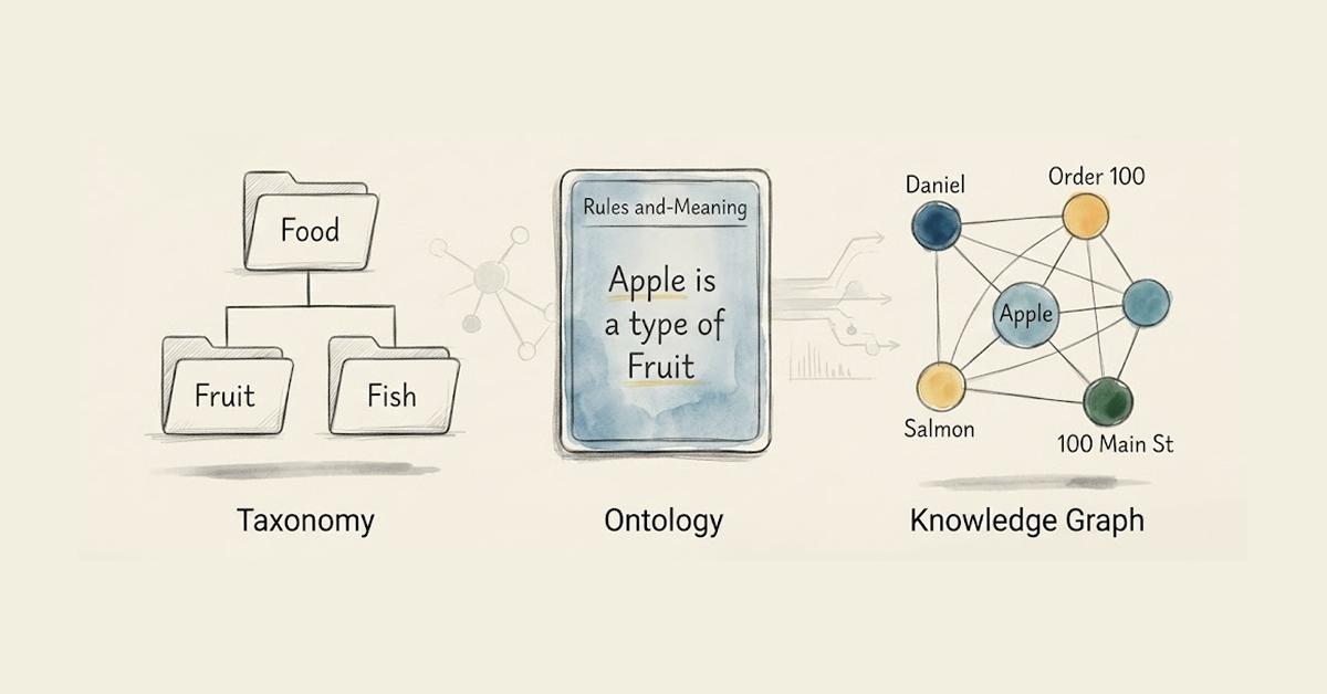
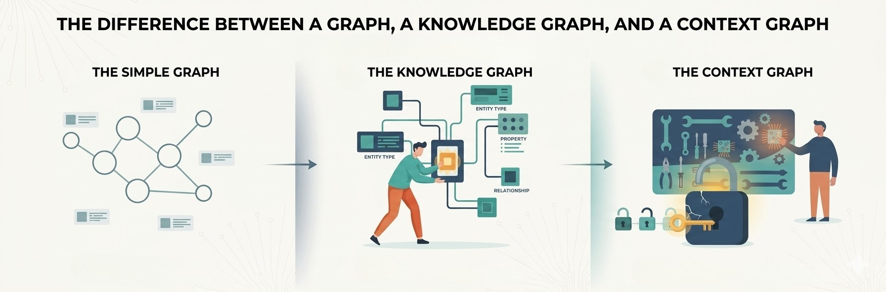
1 of 3: The difference between a graph, a knowledge graph, and a context graph
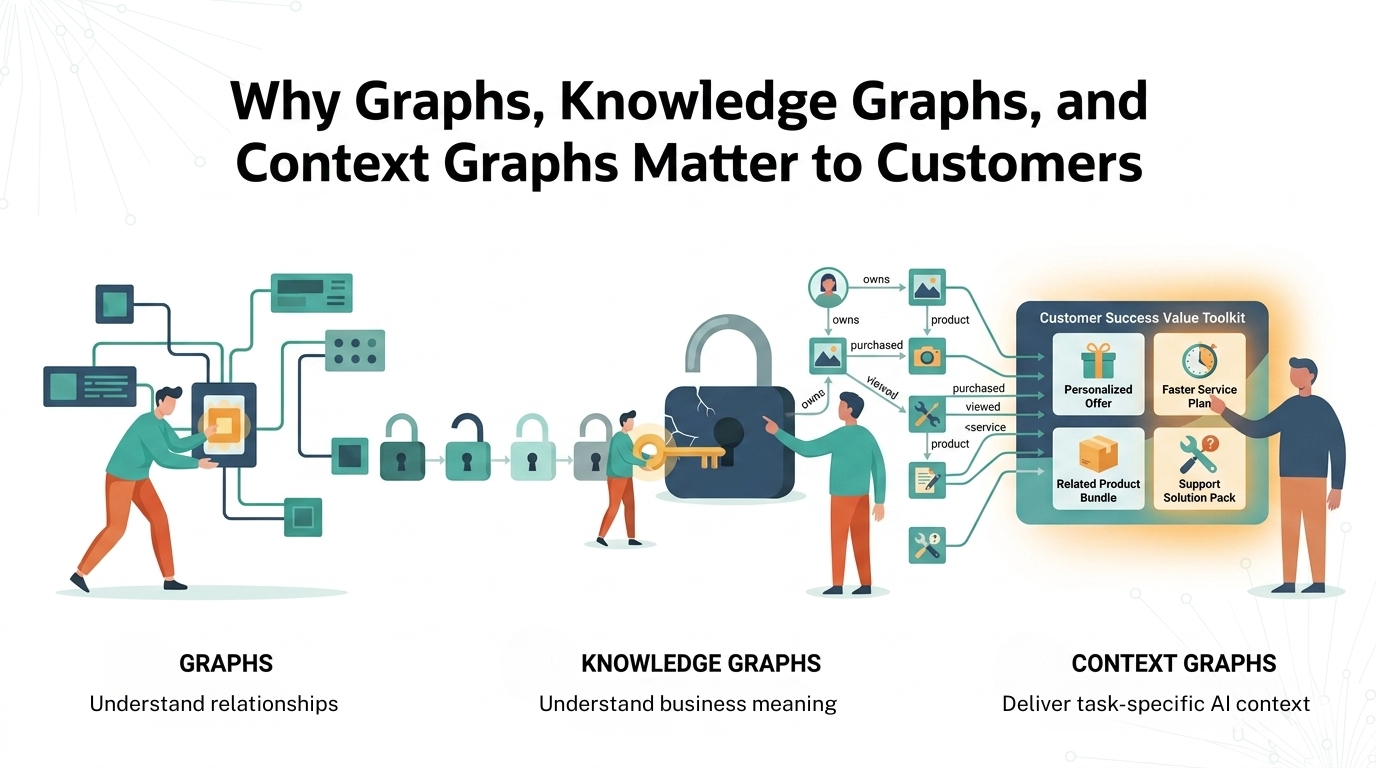
2 of 3: Why graphs, knowledge graphs, and context graphs matter to customers

3 of 3: The graph ecosystem: Bringing connected context to enterprise AI