Performant Queries on Highly Connected, Growing Data

Former CEO, Coshx Labs
22 min read

Editor’s Note: This presentation was given by Michael Wytock at GraphConnect New York in September 2018. At the time Wytock gave this talk, he was the CEO of Coshx Labs, a distributed software consultancy based out of Charlottesville, Virginia.
Presentation Summary
Querying dense, exponentially growing networks in tall, relational databases is often unintuitive and poorly performant. In this post, former CEO of Coshx labs Michael Wytock discusses how to use labels to limit search space as well as how to leverage stored procedures for performance improvements.
Wytock kicks off the post with an explanation of what patents are and why citation relationships are valuable. Then, he discusses the trends in patent data, highlighting how highly connected and quickly growing this data is. He also talks about how they explored this data in Neo4j, as well as the three stages of implementation they experimented with.
Full Presentation: Performant Queries on Highly Connected, Growing Data
My name is Michael Wytock, and I’m the CEO of Coshx Labs.
Before we get into the weeds of things, I want to give a big acknowledgment to one of our clients and partners, M-CAM International. Many of the domain-specific topics that I discuss in this post come from work that we did with them. They’ve graciously allowed us to provide a little bit of insight to you about how their business runs, as well as highlight some of the work that we did in partnership with them to help it run more smoothly.
M-CAM is in the business of intellectual property evaluation. Essentially, they assign value to intellectual property. They also run a fund called the IQ 100, which tracks innovation and is tradable. Like Coshx Labs, M-CAM is also based out of Charlottesville.
Outline
Here’s an outline for the post. The first half will cover a business case study. I’ll be talking about some of the work we did alongside M-CAM. It’ll also lay the foundation for understanding the problems we had to overcome for the technical case study portion, which is the second part of the post.
Getting to Know Patents
Let’s start off with the definition of what a patent is. A patent is a “government-conferred right to exclude others from making, using, or selling an invention for a specified period of time.”
It’s pretty complex – the idea of excluding people from making an invention – but the initial reason for patents was to encourage people to actually share their inventions publicly. By obtaining this exclusive right, you’re more encouraged to actually make the invention for everyone to see.
But, there are a lot of complications when you start tracking the actual data underneath these patents.
If you think of other types of documents, such as academic papers that have citations, those citations come from one document that exists holistically – from its inception throughout its life. It doesn’t change after a 10-year timeframe.
Patents are a bit different than that. They have life cycles, and there are a lot of filings that go through. However, they all capture this one, single invention, though there could be many documents associated with them.
In the United States, if you have an application for a patent, you’d file that with the U.S. Patent and Trademark Office. Then, for roughly 20 years from that filing date, you have the exclusive protection that the patent offers as long as you keep up with all of the prescribed paperwork.
So, you’d start off with this application. Then at some point, you’d fill in paperwork to turn this into a granted patent. Each of these patent documents are different; they’ll all have different document numbers and can change over time.
Legal actions can also be taken on these documents. For example, if an exceedingly broad invention was brought to bare, that invention – through some kind of legal action – may be deemed as needed to be split up to create two separate patents.
We can also seek international equivalencies. This is increasingly important today. Especially in a world with global economies tied together, it’s becoming a lot easier to seek these equivalencies as well.
If you’re in the United States and you want to seek protections in, say, Japan for your patent, there usually has to be a treaty between these two countries which smoothes the way for these types of protections.
You can go to Japan and say, “Hey. Here’s my patent. It’s filed at the U.S. Patent and Trademark Office. I’d like an equivalent patent in Japan.”
There’s a procedure and more paperwork that goes through it. Then, Japan likely has their own process – similar to this one – where you may create multiple documents out of the equivalency process.
At the end of the day, we end up with not just one document for an invention or a piece of intellectual property, but a smattering of documents, which we call a patent family. The European Patent Office has taken great lengths to track these families. Obviously, this problem is more transparent in Europe, where the Eurozone creates different economies that are tied together. In the United States, however, it’s a bit more insulated.
With these international equivalencies, you can now get your single patent shot out to five, 10 or 15 different countries, and companies are starting doing so.
Below is an example of an American patent.
The American patent that we’re looking at here is for a golf putter. These patents usually have these involved names for what’s an everyday item. This one is “Golf Putter Head With Top And Bottom Components Made Of Materials Having Different Densities.” This is pretty standard, as far as how these things are worded.
I’ve pulled out a couple of pieces of data that were of interest to us. There’s obviously the title, filing date, granting date and patent number. You want to know if this patent’s enforced or not. If too much time has gone by, it won’t be.
There’s really two pieces of data that I think are really important for the technical part of this talk: assignees and citations.
Assignees are the entities to which exclusivity is granted. There can be multiple of them. Sometimes it’s the inventor, though in this case it’s not. For example, we have an inventor named David D. Jones here who might’ve worked for the Karsten Manufacturing Corporation. We don’t know the specifics, but we do know that exclusivity is ultimately granted to Karsten.
Then, we have citations, which you’re probably familiar with. They’re related works that you might want to give credit to or are forced to give credit to by someone who reviews the patent. You can also cite across different countries, which is obviously important for enforcement reasons as well.
Project Goal
Now, let’s go back to what the goal of all this really was when we were approached by M-CAM.
I want to unpack a couple of things about this project goal.
First of all, we have performance. M-CAM is mostly concerned with the top 100 largest publicly traded companies in the United States. For companies in the middle of that range, say around 50, it took about a day to crunch those portfolios of patents and assess the value on them.
There’s also an existing algorithm, which was a Java client that accessed a relational database. The algorithm would be checking against some patterns to perform this valuation. These patterns would have scores associated with them, which were used to value the patents.
Then, there’s this idea of value. So, what is a valuable patent? There are many ways we can consider this. Particularly, M-CAM has multiple ways, but by and large, our analysis was mostly concerned with citations. This idea of value through relationships – which in this case are citations – was really important.
So, value equals relationships. If I cite you, what does that mean? If I cite you and you cite someone else, what does that mean? If I don’t cite you and maybe I should have, what does that mean?
We are also talking about patent portfolios here. We’ve talked a lot about individual patents, but large companies own many different patents and they’ve composed a portfolio of intellectual property. I’m sure people have been aware of either legal battles surrounding this, specifically regarding companies who are acquired generally for this intellectual property, either because it’s a threat or because they can leverage it against another company.
We have to think about all of this in aggregate, the key point here being that there’s lots of aggregation that would go on. We have a lot of different documents that need to be aggregated into one. We also have different companies that go by different names and there’s nothing that de-aliases all of those names, so they need to be aggregated into one company.
Then, we have multiple different patents that could be the same in a lot of different companies; they need to be aggregated into one. We also have multiple patents or inventions that this company rightfully holds and they, once again, need to be aggregated into a portfolio that can be analyzed.
Trends in Patent Data
This talk builds and talks about highly connected and exponentially growing data, and I want to be able to quantify that for you a little bit.
As you can see above, we ended up with around 140 million nodes in our database, 100 million of which were patents themselves. The other roughly 40 million nodes were assignees.
The colors above roughly correspond to the snapshot of the graph. Around the outside, we have lots of little assignees that are attached to certain patents. Then, those individual patents are assigned to companies.
Right here in the center is Walmart, or one of the aliases that represents Walmart. As you can see, we have five patents that are all assigned to Walmart.
We also have a couple of citations that are showing. Here, we’re actually showing the one-hop space – in terms of the citations – surrounding these five Walmart patents.
The purple nodes aren’t particularly relevant to this discussion. They’re a way in which we’re aggregating some of these names for other companies and selecting ones we were most interested in. If any companies were not of interest to our analysis, we may throw the data away. These nodes are a sentinel about whether or not we should do that.
There are mainly two types of relationships. The first is one in which an assignment relationship takes the patented document and attaches it to an assignee. The second type is citation relationships between all of these patent documents.
As far as properties go, we had around 900 million properties, which include things like expiration date and issue date. We kept a pretty sparse graph in terms of how much data we put on these properties. There wasn’t free text sitting there on each of these patents.
Below is the same graph blown up a bit.
Here, you can see the Walmart patent in the center and its assignments to these five patents in a one-hop space.
We’re often also concerned with the two-hop space around a patent – we want to know who your patent cites and who that citation cites as well. This is often harder to visualize, but if you imagine pushing these nodes out one frontier further and then pulling in all of the assignees that would be associated there, you can get an idea for how much you can return from one of these queries.
How Highly Connected?
So how highly connected are these data? If you’re looking at Apple – which is in the middle of the road in terms of its raw number of patents held – we end up with about 60,000 patents when running a query matching for Apple.
The citations from Apple balloon quite a bit to over a million patents – 1.4 million or so – which is about a factor of 20 increase. We can tell here that on average, these Apple patents are citing 20 other patents. If we’re looking at the two-hop space, we extend this one step further, ending up with over 200 million patents.
However, if you recall from the “Our Data” image, there are only 100 million patents in the entire dataset. So, how are we returning all of these patents? Well, we’re actually returning the pathways to these patents. Since we have all these citations, we end up returning a lot more data than we initially thought.
This is one of the big issues that was happening with the relational database. As we were doing these joins on the data, we were also returning tons of data. Every time you wanted to go one step further, you were ballooning the amount of data that you had to work through.
A quick disclaimer about Apple: Apple is actually a fairly highly connected portfolio. However, increasingly in recent years, many companies are issuing lots of patents each year. Given that Apple is a relatively young company relative to the others that we would analyze, they’re increasing at a really quick rate.
How Quickly Growing?
Speaking of which, how quickly are patent issuances growing?
In the graph above, we have the number of patents by year. You can see how there’s this curious little plateau that’s been happening recently. There are currently around four million patents being issued per year.
Let’s change the analysis a little bit and look exclusively at patent families per year, shown below. Now you start to see a bit of a different picture.
When we reduce all of those down, we’re seeing how we’re actually getting a lot more independent patent families issued each year. It’s clearly been on the rise in recent years.
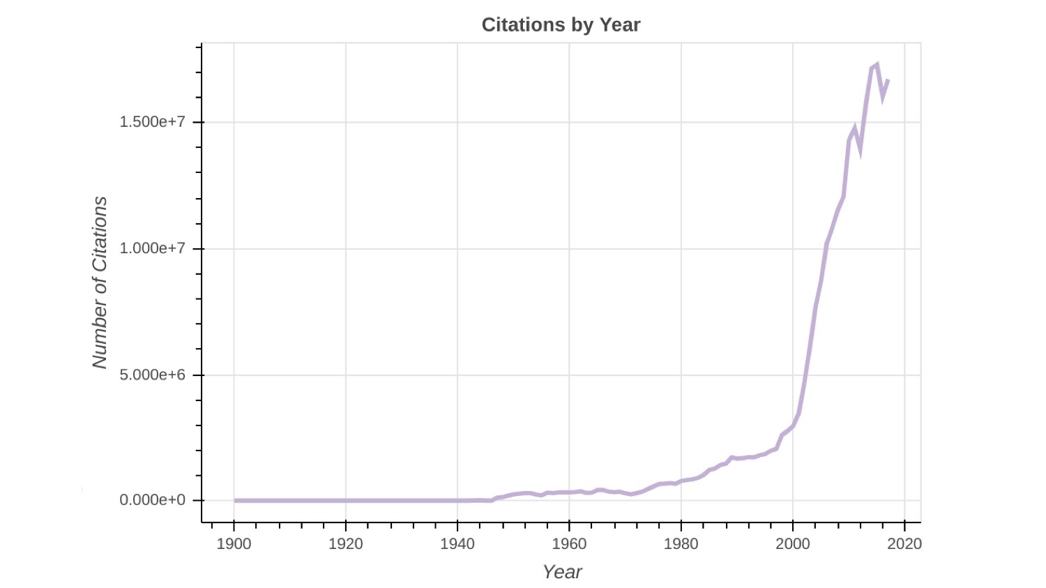
Looking at citations – shown in the graph below – we have around 15 million citations per year.
Again, this appears to be plateauing a little bit.
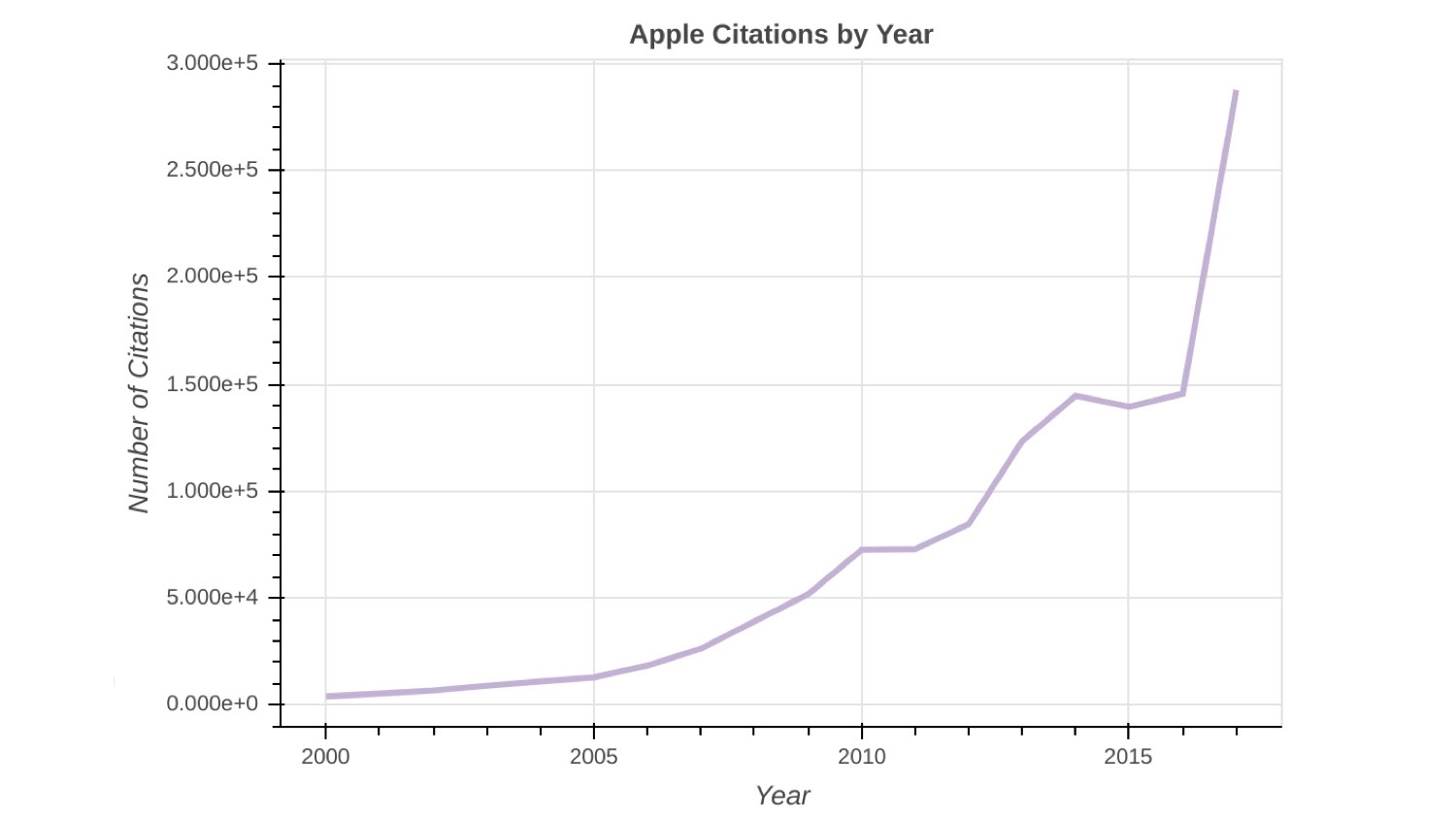
But, if you look at some of the portfolios we were interested in with these very large companies, you can see that they’re citing a lot more people in their patents as well.
This can happen for a variety of reasons, but in many cases, it’s because companies need to cover themselves on a legal basis. That’s one of the reasons they might be doing this.
Algorithmic Challenges
Let’s get to some of the algorithmic challenges we needed to tackle. These were handed to us from the prior analysis that was being done. Once we implemented this in a graph, we wanted to stay true to the analysis that M-CAM already had and then offer some improvements where we could.
The coral-colored node in the graph below is what I’ll call our subject patent. You’d imagine that a company of interest, say Walmart, owns this patent. We want to know things about it, like its value.
There’s a path-finding problem that we have. In this problem, we want to find all of the subject patents owned by Walmart, so we’d look that up. Once we had all of them, we would focus on a single-subject patent. We’d first want to know about its citation network; in this case, we’re talking about a two-hop space.
Then, we would want to find all of these cited patents assignees as well. There are these hidden assignments we’d want to know about, such as who owns these patents. That’s the pathfinding problem – it’s common to a lot of graph issues.
Then there’s pattern matching, another common graph problem. When we look at one of these citation patterns, they have forward citations. We’d have rules about what the score should be assessed for that type of citation pattern and then would have to check against a number of these rules for these patterns. In this way, we’d do lots of pattern matching on a single pathway.
When we were talking about those 200 million pathways we retrieved for Apple, we would then – for every single one of those pathways – do around 10 pattern matches to see whether or not those scores would be good or bad regarding the quality of the patent.
Then, we would have to aggregate and serialize a lot of data. As I mentioned before, we’re dealing with a portfolio here – not an individual patent. So once we got a score for subject patent A, for example, we’d then have to aggregate all other Walmart patents together and produce some kind of intelligible score out of it.
The slide above shows where the data was in a relational database before we got a hold of it.
If you were to do this type of path analysis – to retrieve these paths – in the relational database, something like the following would happen. For example, if we were interested in the US9000000 patent, we’d look it up in the citer column of our database using the global index in the database.
Then if we wanted to go two hops out, we’d have to get another citation, so we’d do a self-join on this table.
For this first citation, let’s say we don’t have a JP citation; somehow, it cites no one, so we’ll dead end there – that’s fine. But for this US94 patent, maybe we have two more. So when we do this join, there’s another global index lookup that has to be done. We get something that looks like the image below.
Right now, what we have is a joined table that’s going to have two forward citations. This is great, though we’re interested in backward citations as well, which creates too many permutations. You’d have to do these joins multiple different ways to figure out where these paths are. It’s a pain.
Why Neo4j?
Now I’ll delve into the reasons why we decided it would be worthwhile to look at a graph database.
First, we get index-free adjacency, instead of global index lookups. If you’re not aware of this term, the idea is really pretty simple: If I’m sitting here at one node, I have references to everyone who’s one hop away from me, so I can just go there. I don’t have to lookup in this huge table with a global index.
There are also undirected queries, so we’re not stuck with bidirectional querying or storing data in multiple different ways. It’s a bit more natural and it also speaks to the last point here.
Last, we have a native graph model instead of the tabular graph model. With the latter model, if you had decided that the three-hop space was important, we would have to go through a huge batch job to change our database structure, perhaps by adding extra columns or doing a lot of compute to get it into the right format.
Moving to Neo4j
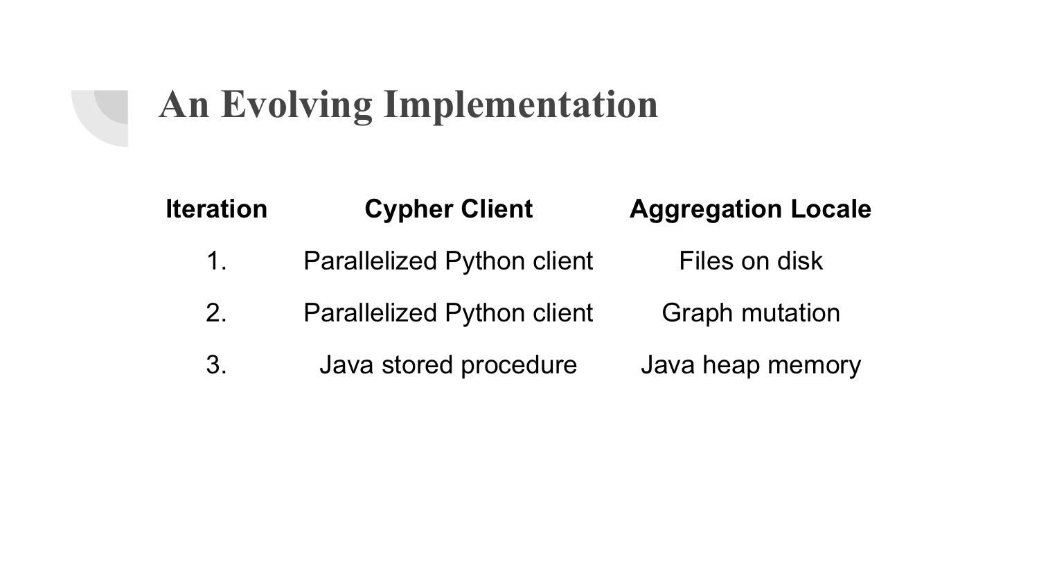
In moving to Neo4j, we had three stages in our implementation, which are shown below.
In the first stage, we used a parallelized Python client and hit the Neo4j database. We did the same thing in the second, but in the third one, we finally went full-in on a Java stored procedure.
What’s interesting about the changes that we made is how we parallelized in the first two versions, as well as where we were doing our aggregation. The aggregation locale for the very first rough-cut version of everything was just files on disks.
Then, for the second version, we thought some indexing might be nice, since the files that held a bunch of data on the disk took forever to aggregate. We knew we had a database next to us, so why not just throw them on the database?
In the final one, we wanted to use all the niceties of being inside of a Turing complete language and working within Java. Therefore, we used a stored procedure and used the memory to do our work.
Version One: Parallel Cypher + Disk Writes
In this first iteration, we were doing parallel Cypher queries with disk writes to write back to files on disks. In the image below, I attempt to show that for a single patent, we had to break these up into pretty granular queries.
We’d match maybe two patterns on those pathways in the first thread and then parallelize across those patterns. We thought that since these queries were lightweight, we wouldn’t end up with a situation where we lockup a thread with a really long query. However, it ended up being a little too easy for the graph database.
If you’re familiar with Python at the global or interpreter lock, dealing with multi-threading inside of Python can be a little messy.
With both our thread and connection pools to our database, there’s a lot of data being sent back and forth and lots of queries initiating and then ending in short time frames. This all became a really chaotic system. Admittedly, it worked pretty well for small portfolios, but as you got bigger, there were just way too many threads being spun up and then later being used again.
The worst part was that our results weren’t indexed. We would just get all the data back, dump them out into these files and then have to aggregate them later.
The lesson here: do more in a query before you start serializing it.
Version Two: Parallel Cypher + Graph Writes
The next time around, we wanted to do two things differently.
First, we wanted to put all of the pattern matches for a single patent into a single thread, so they’d all sit together. Then, the next thread would just be a totally different patent within the same portfolio. In this way, we’d know that we had everything about that one patent already completed.
This made for more demanding queries. In truth, we had to jerry-rig this system, where towards the end, we put off these really gnarly queries that we ran into. We’d kill the query, have a time out and then dedicate a single thread to these really bad ones towards the end. This was all due to memory issues.
Some of the really large patents had these pathological citation pathways, oftentimes self-citing or citing other patents within the same portfolio. There’s a lot that could be said about them, but when you run into them you just know, since these queries are just orders of magnitude longer than others.
There were also lower input/output costs because we were starting to write to Neo4j. We wanted to use the database as a scratch pad because we were already inside of it; we wouldn’t have to pull the data back out to a file, write it, read it again and aggregate in memory in some other paradigm.
There are both good and bad things about this, but in general, consider using Neo4j as a scratchpad. If you’re not sure how you’re going to, pull this data together. You might as well dump it somewhere where you’ll be able to get it out quickly and pivot if necessary. That’s what we did here and we had lower input/output costs than before.
Key Optimizations
Before talking about the historic procedures and how those were used, there are also two other key optimizations that might be useful in some of your own graph queries.
The first one is dynamic label setting. It’s like creating the forbidden fence within your queries.
For us, we’re talking about pathways. With these pathways, at the outset, we could tell all of the patents owned by Walmart fairly easily. Right now they’re represented by relationships, and there are reasons for that instead of a label on the nodes.
What we did when we ran Walmart as a portfolio was find all of the nodes assigned to Walmart and put a label on them indicated that these were the Walmart nodes. When you have thousands – sometimes millions – of nodes that are going to fit that query, you’ll save yourself some pathfinding a bit later if you know you don’t care about these patents in the same way that you care about the other patents.
We limit our search space by doing this, and that’s the key idea. Anything you can do to limit your search space is gonna be useful. In Cypher, with the query planner, sometimes you need to get creative with the ways in which you limit that search space by using labels and things like that. It’s essentially a simple query that basically takes a label and returns the ones that don’t have it.
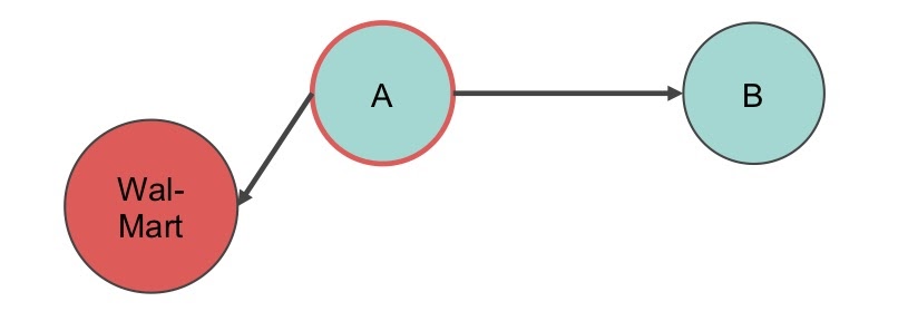
Something akin to that is what we would do. For example, as shown in the image below, we can see how both A and C are assigned to Walmart.
Then we’d basically pull C out once we were able to hop to A, since we knew that C was also assigned to Walmart.
In this way, we can just dump everything that has to do with C out of this and stop traversing this pathway. We don’t want to return it.
The second key optimization is database warmups. If you ever run into this issue, one of a couple things is probably true. Your database might always be on, or it might be a little smaller and there’s no need to pull everything into page cache immediately.
But, you might be dealing with databases that aren’t always on. For us, we were doing a lot of batch jobs; we’d pull in a bunch of patent data and run it on these quarterly changes that happened. However, we would have a lot of uncached data sitting around, and there’s a tremendous performance difference between a cold and warm database.
It’s not always obvious exactly why this is happening, but the idea is that if you don’t run the warmup, your first queries will run it for you. They won’t necessarily do it in a way that’ll help out with query performance.
There’s an APOC call to do this: apoc.warmup.run(true). If you’re not familiar with APOC, you can basically grab a jar file, put it in a correct location, reference it from a CONFIG file and now you have a bunch of usable stored procedures.
One really important – and at the time under-documented – parameter for APOC warmups is pulling properties into the graph. This true parameter pulls those properties into the page cache. It changes things dramatically if you’re looking at any property on a relationship or node during those early queries.
Before warming up, the smallest portfolio we had – the insurance company Progressive – would take around 15 minutes to run. Afterward, it took about 50 seconds or so. The only thing we did to get that was by using the true parameter. Though we were warming up before, we weren’t pulling properties in.
Version Three: Java Stored Procedure
So what’s the deal with Java stored procedures? Why should you do these procedures or why shouldn’t you?
For us, there was no need to manage threads anymore, which was nice. We could also do imperative rather than declarative graph traversals, and we started doing cute things with dynamic label setting.
However, we started to realize that with the way the algorithm had been written before, there were a lot of conditionals. We put these conditionals into case statements inside of Cypher, but case statements in Cypher are often ugly.
We also started to aggregate things inside of Cypher using collects, unwinds, collects again and with-statements, among others. It was turning into modules.
And then we thought, “It’d be pretty nice if we put a function around this part and returned it to this other function, which does the next part.” However, you start losing performance if you have to separate out to different queries for each of those. If you know what this traversal is – and it’s quite an accustomed traversal – you probably should be thinking about using a stored procedure.
In this version, we also got to aggregate things in memory. Obviously, we were doing that before within Cypher, but we just didn’t have too much control over the data structures that were available to us.
Employing Stored Procedures
In giving a bit more of a comparison between Cypher and stored procedures, I will note that at the start of it, my colleague and I thought this would all be a mess, that we would be munging around with Neo4j, implementations and trying to find the correct interface to call.
However, the community was super helpful. They were always on Slack and shot us helpful stuff like jar files that were already hooked up.
I’ll briefly discuss imperative and declarative procedures, which is summarized in the slide below. Cypher is a declarative query language, which is great because most of the optimization is done for you. But, if you’re in a situation where you can avoid a lot of search if you do it in a custom fashion, perhaps you actually want an imperative search. You might find that beneficial for your stored procedure.
In terms of data types, you get maps and lists in Cypher. Obviously, there’s strings as well. However, you can get whatever you need in Java, including native data types.
Moreover, it’s hard to do conditionals inside of Cypher. Inside of Java, however, it’s as easy as it would be if you’re writing the other program.
Then, Cypher often defaults to a depth-first search when you’re trying to find nodes in a graph. At times, you want to escape that and do something conditional – maybe a breadth-first search or a variation of it – in order to optimize the searching you’re doing.
In the image below, I’m not trying to overload you by throwing a bunch of code up. I just want to show how simple it ends up being.
Basically, there’s a big import statement. You’re going to have to set your own schema, so you’ll put in the labels that you have as well as the relationship types that make Neo4j aware of it.
Then there’s this map result, where you have to pull in the type of result you want to return. So, we’re aware that in Cypher, you can return maps. This just means we’ll be able to return this query as a map inside of Cypher.
Further down, we’d pull in the necessary Neo4j classes. You see things like the graph database service. That’s a contextual thing that’s necessary, but then others classes are going to be very familiar, such as nodes, relationships and directions.
In the code below, we see this mocked-up version of finding a two-hop space.
We would use these decorators and call this two-hop space function passing in, which in our case is a patent number. We end up with a pretty nice interface when you’re inside of Cypher.
You’d obviously be using the parameters that get passed in here to use some of these classes that we saw in the previous slide for finding the node, the directionality in relationship from that node conditionally and maybe tabulating some numbers based on that.
Then, at the end of the day, you can return this map result and stream those back out through Neo4j.
Conclusion
For highly connected and quickly growing data, there’s a couple of things that you should keep in mind, such as warming up your database with properties.
Right before I was preparing this post, I saw that the interfaces changed again for that APOC warmup. Now, there’s a couple of other parameters and there might be more things that we can warm up in page cache.
Furthermore, narrow your search space as much as you can, which you can do with labels. You can dynamically set labels and then get rid of them, and also you can use your graph database as a scratchpad.
Also, consider stored procedures if you run into any of these issues. If you know that imperative programming is going to limit your search space tremendously, you may be able to get more performance than Cypher offers.
If Cypher queries are unwieldy and the interface is nasty, the cost isn’t super high to implement the stored procedure. Doing so will be really nice for the usability of your code in the future.
Lastly, if your queries are generating lots of data and you know you’re going to need to aggregate it, that’s another great use case for using the stored procedures. You’ll be able to use those common language constructs inside of Java to perform these aggregations, as opposed to returning data to some intermediary source and write the data to disks.


