Exploring Neo4j Spatial: Path Intersections Using AIS Data

Introduction

In the first two parts of this series — Installation, Data Loading, and Simple Querying and Layer Management, Spatial Filtering, and Intersection — we’ve looked at the Neo4j Spatial plugin, and how to import data and perform simple geospatial operations on point and polygon layers.

Here, I’ll look at how we can use the plugin to analyze Automatic Identification System (AIS) data — a text format used to record vessel location data and metadata transmitted for shipping. I have some AIS data in CSV format, covering a few days of vessel activity in Europe.

If you’re trying these examples yourself, download the sample data. This is a multi-part ZIP archive, so you’ll need a tool to extract the contents.

Create AIS Data Layer

To begin, I create a new layer for the AIS data:

CALL spatial.addLayer('ais_observations', 'wkt',"","")

Then I add the AIS data to that layer using LOAD CSV, calling the spatial.addWKTs procedure in concurrent transactions and adding a node label (ais_transit). (Please see the first two parts for a more detailed discussion of these steps.)

:auto // this is required if you run CALL IN TRANSACTIONS queries using Browser
CALL {
LOAD CSV WITH HEADERS FROM 'file:///ais_all_records.csv' AS row
WITH row.WKT AS wkt, row.MMSI AS mmsi, row.DATE AS date, row.TIME as time,
row.SPEED AS speed, row.NAME AS name, row.DESTINATION AS destination,
row.AISTYPE_1 AS aistype, row.ETA AS eta
WHERE wkt IS NOT NULL AND wkt <> ''
CALL spatial.addWKTs('ais_observations', [wkt]) YIELD node
SET node:ais_transit,
node.name = name,
node.mmsi = mmsi,
node.time = time,
node.date = date,
node.speed = speed,
node.destination = destination,
node.aistype = aistype,
node.eta = eta
RETURN count(*) AS _
} IN CONCURRENT TRANSACTIONS OF 500 ROWS
ON ERROR CONTINUE
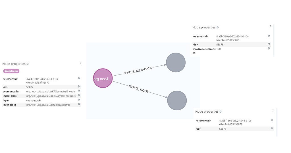
FINISH

We should test whether the data loaded correctly. To recap from the previous blog, we can query the spatial layer by traversing the root-child-reference structure of the R-tree index, like this:

CALL spatial.layer("ais_observations") YIELD node AS layerNode
MATCH (layerNode)-[:RTREE_ROOT]-()-[:RTREE_CHILD*]-()-[:RTREE_REFERENCE]-(n)
WHERE n.name CONTAINS "SAMSKIP"
RETURN n.geometry, n.time ORDER BY n.time DESC LIMIT 1
This query finds the most recent location of a vessel called 'SAMSKIP', and completes in 29ms. 
Here is the same query, using the 'ais-transit' label that we added when loading the data.
MATCH (n:ais_transit)
WHERE n.name CONTAINS "SAMSKIP"
RETURN n.geometry

This query returns in 5 ms:

╒═══════════════════════════╤═══════════╕
│n.geometry │n.time │
╞═══════════════════════════╪═══════════╡
│"POINT (-0.50288 50.49736)"│"18:31:03Z"│
└───────────────────────────┴───────────┘

This is a useful reminder to always set a label when loading spatial data via the Neo4j Spatial plugin. You’ll thank yourself later!

AIS data contains vessel tracking observations. Each row contains a single observation of a vessel location, its name, and Maritime Mobile Service Identity (MMSI) number, and various properties, such as vessel speed, heading, destination, as well as a code for the vessel type (cargo, passenger ferry, etc).

Plotting AIS data on a map shows the individual observation points, but these points need to be connected to recreate the vessel’s journey (or transits). My plan is first to connect all the individual observations for each vessel with a NEXT and PREVIOUS relationship, thereby encoding each vessel’s journey, observation by observation, in the graph.

This will entail ordering the data first on MMSI (the unique vessel identifier code), then on Date, and then on DateTime. The imported data treats the date and time values as strings, which can’t be ordered, so we first have to convert these values to the appropriate data type:

MATCH (n:ais_transit)
SET n.date = datetime(n.date), n.time = time(n.time)
RETURN count(n)
I can then order the data and create the desired relationships:
MATCH (n:ais_transit)
ORDER BY n.mmsi, n.date, n.time // Ensure correct chronological ordering
WITH n.mmsi AS mmsi, collect(n) AS nodes // Collect all nodes for each MMSI in order
UNWIND range(0, size(nodes)-2) AS i
WITH nodes[i] AS a, nodes[i+1] AS b
MERGE (a)-[:NEXT]->(b)
MERGE (b)-[:PREVIOUS]->(a)

This created 61,168 relationships and completed after 630 ms.

Let’s see how this looks in the data. We’ll query on the path pattern, as we want to return some complete paths and see the new relationships we generated:

CALL spatial.layer("ais_observations") YIELD node AS layerNode
MATCH p = (layerNode)-[:RTREE_ROOT]-()-[:RTREE_CHILD*]-()-[:RTREE_REFERENCE]-(n)
RETURN p

We see that the vessel transits are now connected, and we can look at one of those transits in more detail:

MATCH (n:ais_transit)
WHERE n.name CONTAINS "VN PARTISAN"
RETURN n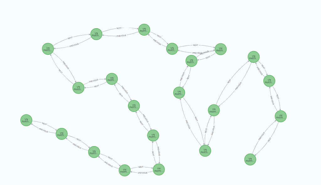

What we did here is essentially recreate the separate transits or journeys recorded for each vessel as a discrete subgraph. Each node possesses a point location in its geometry property, so this is starting to look a bit more like a polyline than the collection of disconnected points observations loaded from our AIS file.

If all we want to do is to visualize the journeys, we’re done. Most likely though, we need to do some more geo-processing to determine the geographic characteristics of those naval paths.

Convert to Polyline

So now we’re going to convert this into a proper POLYLINE (or LINESTRING) feature and store that in a new layer. Converting this data to polylines will let us perform more complex types of geo-processing, such as calculating where transits intersect each other or intersect defined areas of interest.

Again, we apply the steps from the first two parts. First, we create our WKT spatial layer in the usual manner:

CALL spatial.addLayer('ais_uk_lines', 'wkt',"","")

Then we take collections of the :ais_transit nodes we created, then group, sort, and collect their geometries to build a WKT LINESTRING. We create a new set of nodes with an :ais_line_staging label, with each node having a WKT LINESTRING geometry property, containing a discrete, complete AIS transit. For each node, we also calculate the start date and time, destination, and a derived average speed for the transit.

:auto
CALL {
MATCH (spatialNode:ais_transit)
RETURN spatialNode.mmsi AS mmsi,
spatialNode.name AS name,
spatialNode.speed AS speed,
spatialNode.date AS date,
spatialNode.time AS time,
spatialNode.geometry AS geometry
} IN CONCURRENT TRANSACTIONS OF 100 ROWS ON ERROR CONTINUE
// 2. Group by vessel and collect attributes
WITH mmsi, name,
collect({
geom: geometry,
date: date,
time: time,
speed: CASE WHEN speed IS NOT NULL AND speed <> '' THEN toFloat(speed) ELSE NULL END
}) AS records
// 3. Keep only groups with 2+ points
WHERE size(records) >= 2
// 4. Sort the records by date and time
WITH mmsi, name,
[rec IN records | [rec.date, rec.time, rec.geom, rec.speed]] AS rawData
UNWIND rawData AS row
WITH mmsi, name, row
ORDER BY mmsi, name, row[0], row[1]
// 5. Collect the sorted values
WITH mmsi, name,
collect(row[2]) AS geomList,
collect(row[0]) AS dates,
collect(row[1]) AS times,
[sp IN collect(row[3]) WHERE sp IS NOT NULL] AS speedsFiltered
// 6. Build WKT LINESTRING with coordinate pairs (x y) and compute average speed
WITH mmsi, name,
"LINESTRING(" + reduce(txt = "", val IN geomList |
CASE WHEN txt = "" THEN
// Extract coordinates from "POINT (x y)" string
substring(val, 7, size(val) - 8) // Remove "POINT (" and ")"
ELSE txt + ", " + substring(val, 7, size(val) - 8) END) + ")" AS linestringWKT,
head(dates) AS firstDate,
last(dates) AS lastDate,
head(times) AS firstTime,
last(times) AS lastTime,
CASE
WHEN size(speedsFiltered) > 0
THEN reduce(s = 0.0, v IN speedsFiltered | s + v) / size(speedsFiltered)
ELSE null
END AS avg_speed
// 7. Assign transit_id and write flat properties to :ais_line_staging
ORDER BY mmsi, firstDate, firstTime
WITH collect([mmsi, name, linestringWKT, firstDate, lastDate, firstTime, lastTime, avg_speed]) AS allData
UNWIND range(0, size(allData) - 1) AS idx
WITH idx AS transit_id, allData[idx] AS data
WITH
transit_id,
data[0] AS mmsi,
data[1] AS name,
data[2] AS linestringWKT,
data[3] AS firstDate,
data[4] AS lastDate,
data[5] AS firstTime,
data[6] AS lastTime,
data[7] AS avg_speed
CREATE (n:ais_line_staging {
transit_id: transit_id,
mmsi: mmsi,
name: name,
linestringWKT: linestringWKT,
firstDate: firstDate,
lastDate: lastDate,
firstTime: firstTime,
lastTime: lastTime,
avg_speed: avg_speed
})
RETURN n.transit_id, n.mmsi, n.linestringWKT
Finally, we will load the ais_line_staging WKT LINESTRING geometry into a new ais_transits spatial layer, also adding the properties from the relevant ais_line_staging node.
Create a layer to hold the polyline/linestring geometry:
CALL spatial.addLayer('ais_transits', 'wkt',"","")
Then load the data from the ais_line_staging nodes:
MATCH (t:ais_line_staging)
WHERE t.transit_id IS NOT NULL AND t.linestringWKT IS NOT NULL
WITH
t.transit_id AS transit_id,
t.linestringWKT AS wkt,
t.mmsi AS mmsi,
t.name AS name,
t.firstDate AS firstDate,
t.lastDate AS lastDate,
t.firstTime AS firstTime,
t.lastTime AS lastTime,
t.avg_speed AS avg_speed
// Step 2: Create spatial node in uk_ais_lines with label :ais_uk_transit_lines and assign properties
CALL spatial.addWKT('ais_transits', wkt) YIELD node
SET node.transit_id = transit_id,
node.mmsi = mmsi,
node.name = name,
node.firstDate = firstDate,
node.lastDate = lastDate,
node.firstTime = firstTime,
node.lastTime = lastTime,
node.avg_speed = avg_speed
SET node:ais_uk_transit_lines
RETURN transit_id, node
Now, we can clean up after ourselves and delete those staging nodes:
MATCH (t:ais_line_staging)
DETACH DELETE t

Test the Geometry

And finally, we should test that our LINESTRING geometry loaded properly. An obvious test for AIS transits is to query for intersections with a polygon. This could be useful for detecting when a vessel enters an exclusion zone (such as a trawler entering a protected area or a commercial vessel sailing too close to a windfarm). For this test, I created a simple exclusion zone in the English Channel and saved it as a CSV with polygon geometry in a WKT column.

So we follow the now-familiar process:

CALL spatial.addLayer('exclusion', 'wkt',"","")

Then:

LOAD CSV WITH HEADERS FROM 'file:///exclusion.csv' AS row
WITH row.WKT AS wkt, row.zone AS zone
WHERE wkt IS NOT NULL AND wkt <> '' // Skip empty WKT values
CALL spatial.addWKTs('exclusion', [wkt]) YIELD node
SET node.zone = zone, node:exclusion
RETURN node;

Then we use the spatial.intersects procedure to test for AIS transits that cross my exclusion zone:

MATCH (spatialNode:transit)
//WHERE spatialNode.name CONTAINS "VN PARTISAN"
CALL spatial.intersects("exclusion", spatialNode.geometry) YIELD node
RETURN spatialNode.name, spatialNode.transit_id ORDER BY spatialNode.transit_id DESC

This works well enough and will tell us if our transits cross the exclusion zone. However, a more useful query would be to ask where our vessel entered the exclusion zone. Unfortunately, that’s beyond the abilities of the spatial.intersects procedure.

Summary

We used AIS data to visualize and investigate vessels’ journeys. We also reached a point where the current Neo4j Spatial plugin functionality isn’t sufficient for our investigation, so in the next part, we’ll look at how we can extend the capabilities of the plugin with a simple, custom plugin.

---

Exploring Neo4j Spatial: Path Intersections Using AIS Data was originally published in Neo4j Developer Blog on Medium, where people are continuing the conversation by highlighting and responding to this story.