Agentic Graph Analytics With External MCP Providers and Neo4j

Graph ML and GenAI Research, Neo4j
8 min read

Building modular graph analytics pipelines with Neo4j Aura Graph Analytics and external data sources
Neo4j Aura Graph Analytics is a serverless offering for running graph algorithms in the cloud. While it can connect to existing Neo4j databases, it also supports a stand-alone mode where the data source is not Neo4j at all. You can load data directly from pandas DataFrames, run algorithms like PageRank or community detection, and stream results back without ever touching a Neo4j database. This is useful when your data lives in a relational database, a data warehouse, or just CSV files, and you want to apply graph algorithms without setting up graph infrastructure.
I wanted to see what it would take to expose these capabilities to LLM agents through an MCP server, and it turned out there are some interesting challenges to solve, including:
- How to get data from external sources without building and maintaining a separate integration for each data provider
- How to keep the actual graph data out of the LLM context, which would quickly get overwhelmed
- If it makes sense to group algorithms into higher-level tools rather than exposing each one individually
In this blog post, I’ll walk through what I learned while building this MCP server. The code is available on GitHub.
Note: This is a proof-of-concept implementation and is not officially supported or intended for production use.
Integrating External Data Sources
One approach to supporting external data sources would be to build dedicated integrations for each provider: one for Snowflake, one for BigQuery, etc. But that means writing and maintaining a lot of code, and every new data source requires additional work. Instead, I wanted to see if we could piggyback on existing MCP servers that already know how to talk to these systems. It turns out that mounting existing MCP implementations from external data providers seems to be a good idea.

For this experiment, I used Supabase as the external data provider. Supabase already has an MCP server that exposes tools for executing SQL queries, listing tables, and other database operations. Rather than reimplementing all of that, our Neo4j Aura Graph Analytics MCP server can dynamically mount the Supabase MCP server when a Supabase API key is provided in the environment.
# Initialize MCP server
mcp = FastMCP(
    name="neo4j-gds",
)

if supabase_access_token:
    logger.info(f"Using Supabase MCP")
    # Create the stdio transport
    supabase_transport = StdioTransport(
        command="npx",
        args=[
            "-y",
            "@supabase/mcp-server-supabase@latest",
            "--access-token",
            supabase_access_token
        ]
    )

    # Pass transport directly - ProxyClient is created automatically
    supabase_proxy = FastMCP.as_proxy(
        supabase_transport,
        name="Supabase"
    )
    # Mount the proxy
    mcp.mount(supabase_proxy, prefix="supabase")
No API key, no Supabase tools. This pattern scales nicely: You could add support for other providers the same way, mounting their MCP servers conditionally based on available credentials.
The second challenge is avoiding data flow through the LLM. If the agent fetches rows from Supabase and passes them to another tool to load into Graph Data Science, all that data ends up in the context window. For small datasets, that might be fine, but it doesn’t scale. The solution is to implement a single tool that internally handles the entire pipeline of fetching the dataset and constructing an Aura graph projection.
if supabase_access_token:
    @mcp.tool(
            name=namespace_prefix + "load_gds_graph_from_supabase",
            annotations=ToolAnnotations(
                title="Load GDS Graph from Supabase",
                readOnlyHint=False,
                destructiveHint=False,
                idempotentHint=True,
                openWorldHint=True,
            ),
        )
    async def load_gds_graph_from_supabase(
        project_id: str = Field(
            ...,
            description="Supabase project ID"
        ),
        nodes_query: str = Field(
            ...,
            description="SQL query to fetch nodes. Must return a 'nodeId' column (integer) and optional 'labels' column (string or array) and numeric properties. Use double quotes to preserve case for aliasing. Example: SELECT id as \"nodeId\", type as \"labels\" FROM nodes"
        ),
        relationships_query: str = Field(
            ...,
            description="SQL query to fetch relationships. Must return 'sourceNodeId' and 'targetNodeId' columns (integers), optional 'relationshipType' column (string), and numeric properties. Use double quotes to preserve case for aliasing. Example: SELECT source_id as \"sourceNodeId\", target_id as \"targetNodeId\", type as \"relationshipType\" FROM edges"
        ),
        graph_name: str = Field(
            default="graph",
            description="Name for the graph in GDS. Default is 'graph'"
        ),
        undirected: bool = Field(
            default=False,
            description="If True, all relationship types will be treated as undirected. Default is False (directed)."
        ),
        session_name: Optional[str] = Field(
            default=None,
            description="Name for the GDS session. If not provided, a default name will be generated"
        ),
        memory: Optional[str] = Field(
            default=None,
            description="Memory allocation for the session (e.g., '4GB'). If not provided, will be estimated based on graph size"
        ),
        ttl_hours: int = Field(
            default=5,
            description="Time-to-live for the session in hours. Default is 5 hours"
        )
    ) -> list[ToolResult]:
        """Load a graph into Neo4j GDS by fetching data from Supabase via SQL queries with support for node labels, relationship types, and undirected relationships."""

... code implementation ...
The load_gds_graph_from_supabase tool takes SQL queries for nodes and relationships, calls the Supabase execute_sql tool under the hood, and loads the results directly into a Graph Data Science session. The LLM never sees the actual data, only the queries and the confirmation that the graph was loaded.
Another benefit of using the execute_sql tool under the hood for projecting nodes and relationships is that the LLM can perform any needed data transformations using the SQL query language.
Grouping Algorithms
The third design decision was around how to expose Graph Data Science algorithms to the LLM. Neo4j’s Graph Data Science library includes dozens of algorithms across different categories: centrality, community detection, pathfinding, similarity, and more. You could expose each one as a separate tool, but that creates a problem as it bloats the tool catalog that the LLM has to choose from, making tool selection harder and costing a bunch of tokens.
Instead, I grouped algorithms by their semantic purpose. Rather than having four separate tools for run_pagerank, run_betweenness, run_degree, and run_closeness, there’s a single run_centrality_algorithm tool that takes the algorithm name as a parameter. This keeps the tool count manageable while still giving the LLM full control over which specific algorithm to use.
@mcp.tool(
    name=namespace_prefix + "run_centrality_algorithm",
    annotations=ToolAnnotations(
        title="Run Centrality Algorithm",
        readOnlyHint=True,
        destructiveHint=False,
        idempotentHint=True,
        openWorldHint=True,
    ),
)
async def run_centrality_algorithm(
    algorithm_name: Literal["pagerank", "betweenness", "degree", "closeness"] = Field(
        ...,
        description="Name of the centrality algorithm to run. Options: 'pagerank', 'betweenness', 'degree', 'closeness'"
    ),
    session_name: str = Field(
        ...,
        description="Name of the GDS session"
    ),
    graph_name: str = Field(
        ...,
        description="Name of the graph to run the algorithm on"
    )
The same pattern applies to community detection: one tool for run_community_detection_algorithm that supports Louvain, Leiden, Label Propagation, and Weakly Connected Components (WCC). The LLM can reason about what type of analysis it needs to perform (“I need to find communities” or “I need to measure influence”) and pick the specific algorithm that best fits the task.
Test Run
To test the setup, I created a Supabase project with two tables: one for Persons and another for friendships. I then configured my Claude Desktop with the following MCP server credentials:
{
  "mcpServers": {
    "neo4j-aura-graph-analytics": {
      "command": "uv",
      "args": [
        "--directory",
        "/path/to/mcp-aura-gds-managed/mcp-neo4j-aura-gds-standalone",
        "run",
        "mcp-neo4j-aura-gds-standalone",
        "--transport",
        "stdio",
        "--namespace",
        "dev"
      ],
      "env": {
        "CLIENT_ID": "",
        "CLIENT_SECRET": "",
        "SUPABASE_ACCESS_TOKEN": ""
      }
    }
  }
}
Next, I asked Claude to load the friendship graph into a Graph Data Science session and run PageRank and WCC on it. Claude performed four steps to identify the data in Supabase before loading the Graph Data Science graph with the following parameters:

After a total of nine steps, the workflow finished, and the LLM presented the results.

For centrality algorithms, we stream the top 10 results to the LLM, while for community detection algorithms, we return aggregate statistics.
Summary
This proof of concept shows that you can build modular graph analytics pipelines by composing existing MCP servers rather than reinventing integrations from scratch. By mounting external providers like Supabase, keeping raw data out of the LLM context, and grouping algorithms semantically, you end up with a system where an LLM agent can fetch data from external sources, run graph algorithms on it, and get insights back without ever touching a dedicated graph database or overwhelming the context window with rows of data.
The approach scales by dynamically mounting different MCP servers; swap Supabase for Snowflake or BigQuery and the architecture stays the same. For exploratory workflows where the data isn’t already in graph form, this architecture provides a lightweight way to bring graph algorithms into agentic workflows.
The code is available on GitHub.
Essential GraphRAG
Unlock the full potential of RAG with knowledge graphs. Get the definitive guide from Manning, free for a limited time.
Agentic Graph Analytics With External MCP Providers and Neo4j was originally published in Neo4j Developer Blog on Medium, where people are continuing the conversation by highlighting and responding to this story.


