Finding Hidden Bottlenecks in Flight Networks with Aura Graph Analytics on Databricks

Why does bad weather in Atlanta end up canceling your flight all the way in Seattle? That’s the reality of a network. Air travel depends on a small number of highly connected hubs, and when one is disrupted, the effects cascade across the system, exposing dependencies you can’t see in a simple schedule.

Previously, you learned about how Aura Graph Analytics interfaces with Databricks. In this post, you’ll walk through a real example: loading flight route data in Databricks, projecting it as a graph with Aura Graph Analytics, and using a community detection algorithm (Weakly Connected Components), a centrality algorithm (Betweenness), and a pathfinding algorithm (Dijkstra’s Shortest Path) to find the hidden risky bottlenecks in the flight network — and reroute around them on the fly.

Mission Control

You will play the role of a data scientist working in logistics for a top international shipping company. Your team is tasked with monitoring and responding to changes in flights and how that might affect the flow of air cargo. 

It will be helpful to have an all-up view of the flight grid and a way to reroute traffic or find existing alternative flights if weather knocks an airport out of commission temporarily.

Getting and Cleaning the Data

First, you need some data and a place to put it. Start by creating a demo database.

%sql
CREATE DATABASE IF NOT EXISTS hive_metastore.flights_demo;Code language: CSS (css)

Then add in airline routes from OpenFlights and save them as a delta table in our flights_demo database.

import requests
from pyspark.sql.functions import col

# Download the file content
response = requests.get("https://raw.githubusercontent.com/jpatokal/openflights/master/data/routes.dat")
content = response.text

# Write to DBFS
dbutils.fs.put("dbfs:/tmp/routes.dat", content, overwrite=True)

# Read into a dataframe
df = spark.read.csv(
    "dbfs:/tmp/routes.dat",
    header=False,
    inferSchema=True,
    sep=","
)

# Rename columns
df = df.toDF(
    "airline", "airline_id", "src_airport", "src_airport_id",
    "dst_airport", "dst_airport_id", "codeshare", "stops", "equipment"
)

# Save as a Delta table
df.write.format("delta").mode("overwrite").saveAsTable("hive_metastore.flights_demo.routes")

print("Done!")Code language: PHP (php)

Then you will do the same with the airports’ data!

# Download airports data
response = requests.get("https://raw.githubusercontent.com/jpatokal/openflights/master/data/airports.dat")
content = response.text

dbutils.fs.put("dbfs:/tmp/airports.dat", content, overwrite=True)

df_airports = spark.read.csv(
    "dbfs:/tmp/airports.dat",
    header=False,
    inferSchema=True,
    sep=","
)

# Rename columns
df_airports = df_airports.toDF(
    "airport_id", "name", "city", "country", "iata", "icao",
    "latitude", "longitude", "altitude", "timezone", "dst",
    "tz_database", "type", "source"
)

# Save as Delta table
df_airports.write.format("delta").mode("overwrite").saveAsTable("hive_metastore.flights_demo.airports")

print("Done!")Code language: PHP (php)

Creating a Session

Now that you have your data, you need a quick and flexible way to handle it. With Aura Graph Analytics, you can easily find connected insights from our Deltatables in Databricks. First, download the package:

%pip install graphdatascience

Next, load all your Aura credentials. 

clientid = dbutils.secrets.get(scope="demo", key="clientid")
clientsecret = dbutils.secrets.get(scope="demo", key="clientsecret")
tenantid = dbutils.secrets.get(scope="demo", key="tenantid")Code language: JavaScript (javascript)

Then create a session. (Please note that you will need an Aura account with Graph Analytics to follow along)

from graphdatascience.session import GdsSessions, AuraAPICredentials, AlgorithmCategory, CloudLocation
from datetime import timedelta
import pandas as pd

sessions = GdsSessions(api_credentials=AuraAPICredentials(clientid, clientsecret, tenantid))

name = "my-new-session-flights"
memory = sessions.estimate(
    node_count=20,
    relationship_count=50,
    algorithm_categories=[AlgorithmCategory.CENTRALITY, AlgorithmCategory.NODE_EMBEDDING],
)
cloud_location = CloudLocation(provider="gcp", region="europe-west1")

gds = sessions.get_or_create(
    session_name=name,
    memory=memory,
    ttl=timedelta(hours=5),
    cloud_location=cloud_location,
)Code language: JavaScript (javascript)

Then clean the data to the right format. You will need a table for nodes and a table for relationships.

For The Table Representing Nodes:

The first column should be called nodeId, which represents the ids for each node in your graph.

For The Table Representing Relationships:

You need to have columns called sourceNodeId and targetNodeId. These will tell Graph Analytics the direction of the relationships, which in this case means:

• The starting airport (sourceNodeId) and
• The ending airport (targetNodeId)

# Edges — routes
rels_pd = spark.table("hive_metastore.flights_demo.routes") \
    .select("src_airport_id", "dst_airport_id") \
    .toPandas() \
    .rename(columns={
        "src_airport_id": "sourceNodeId",
        "dst_airport_id": "targetNodeId"
    })

rels_pd["relationshipType"] = "ROUTE"

# Cast to int
rels_pd["sourceNodeId"] = pd.to_numeric(rels_pd["sourceNodeId"], errors="coerce").astype("Int64")
rels_pd["targetNodeId"] = pd.to_numeric(rels_pd["targetNodeId"], errors="coerce").astype("Int64")
rels_pd = rels_pd.dropna(subset=["sourceNodeId", "targetNodeId"])

# Build nodes from airports that exist in routes
airports_in_routes = set(rels_pd["sourceNodeId"]).union(set(rels_pd["targetNodeId"]))

nodes_pd = spark.table("hive_metastore.flights_demo.airports") \
    .select("airport_id") \
    .toPandas() \
    .rename(columns={"airport_id": "nodeId"})

nodes_pd["nodeId"] = pd.to_numeric(nodes_pd["nodeId"], errors="coerce").astype("Int64")
nodes_pd = nodes_pd.dropna(subset=["nodeId"])
nodes_pd = nodes_pd[nodes_pd["nodeId"].isin(airports_in_routes)]

# Filter rels to only valid node IDs (catches any stragglers like 7167)
valid_ids = set(nodes_pd["nodeId"])
rels_pd = rels_pd[
    rels_pd["sourceNodeId"].isin(valid_ids) &
    rels_pd["targetNodeId"].isin(valid_ids)
]

print(f"Nodes: {len(nodes_pd)}, Edges: {len(rels_pd)}")Code language: PHP (php)

Note: to keep our example simple, the data will be cleaned to only include airports with associated flight paths from OpenFlights. Additionally, since you are playing the role of a data scientist at a shipping company, you won’t distinguish between passenger and cargo flights. 

Creating a Graph Projection

Next, you create a graph projection using the gds.graph.construct method. This will create an in-memory graph to run algorithms against.

graph_name = "flights-graph"
if gds.graph.exists(graph_name)["exists"]:
    # Drop the graph if it exists
    gds.graph.drop(graph_name)
    print(f"Graph '{graph_name}' dropped.")

G = gds.graph.construct(graph_name, nodes_pd, rels_pd)Code language: PHP (php)

To visualize what your graph looks like, install the neo4j-viz package.

%pip install neo4j-viz

You are going to look at a subset of our graph here (200 nodes). The code to run this will be very similar to what is necessary to construct a graph. You need a dataframe of nodes and a dataframe of edges. Because you are only looking at a subset, the graph will be mostly disconnected.

from neo4j_viz import Node, Relationship, VisualizationGraph
airports_pd = spark.table("hive_metastore.flights_demo.airports") \
    .select("airport_id", "name", "city", "country", "iata") \
    .toPandas()

airports_pd["airport_id"] = pd.to_numeric(airports_pd["airport_id"], errors="coerce").astype("Int64")
sample = rels_pd.sample(200)
sample_node_ids = set(sample["sourceNodeId"]).union(set(sample["targetNodeId"]))
sample_airports = airports_pd[airports_pd["airport_id"].isin(sample_node_ids)]

nodes = [
    Node(
        id=int(row["airport_id"]),
        caption=str(row["iata"]) if row["iata"] else str(row["airport_id"])
    )
    for _, row in sample_airports.iterrows()
]

rels_viz = [
    Relationship(
        source=int(row["sourceNodeId"]),
        target=int(row["targetNodeId"])
    )
    for _, row in sample.iterrows()
]

VG = VisualizationGraph(nodes=nodes, relationships=rels_viz)
VG.render()
Code language: PHP (php)

Validating The Data

Before you start rerouting cargo, you need to know what you’re working with. A flight network is only useful if it’s actually connected — gaps in the data mean blind spots in our operations, and in logistics, blind spots cost money.

First run Weakly Connected Components (WCC) against the graph projection. Think of it as a systems check: are you looking at one coherent flight grid, or a patchwork of disconnected islands? If a cluster of airports isn’t reachable from the rest of the network, no algorithm in the world will find a reroute through them, and you need to know that before a weather event forces our hand.

# Run WCC in stream mode
components = gds.wcc.stream(G)

component_counts = components.groupby("componentId")["nodeId"].count().reset_index() \
    .rename(columns={"nodeId": "count"})

component_counts.groupby("count")["componentId"].count().reset_index() \
    .rename(columns={"count": "component_size", "componentId": "number_of_components"}) \
    .sort_values("component_size", ascending=False)Code language: PHP (php)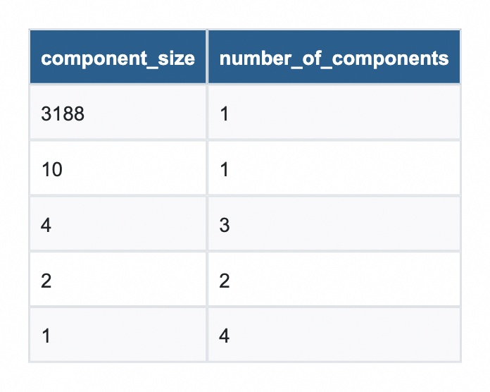

From this, you can see that nearly all of the airports are part of a single component with a size of 3,188. Looks like you are good to go!

Finding a Bottleneck

Now that you are confident in the graph projection, let’s find which airports are bottlenecks for operations. If the weather were to affect one of our major hubs, it could ripple down the line and affect routes.

To find them, run Betweenness Centrality against our graph projection. The algorithm works by calculating how frequently each airport appears on the shortest path between every pair of airports in the network. The higher the score, the more routing traffic depends on that single node, and the bigger the operational risk if it goes down.

The fifth-largest score belongs to an airport that may surprise travelers but is quite expected for air cargo: Ted Stevens Anchorage International Airport. Few passengers lay over here anymore, but it is a very common stop for cargo planes to refuel on their way from Asia to North America.

# Run Betweenness Centrality
betweenness = gds.betweenness.stream(G).sort_values("score", ascending=False)

# Pull airports from Spark to Pandas
airports_pd = spark.table("hive_metastore.flights_demo.airports") \
    .select("airport_id", "name", "city", "country", "iata") \
    .toPandas()

airports_pd["airport_id"] = pd.to_numeric(airports_pd["airport_id"], errors="coerce").astype("Int64")

# Join on nodeId
result = betweenness.merge(airports_pd, left_on="nodeId", right_on="airport_id", how="left") \
    .drop(columns="airport_id") \
    [["name", "city", "country", "score"]]Code language: PHP (php)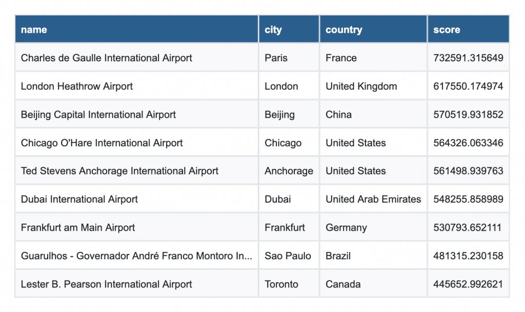

Shortest Paths

That raises the question: what would happen if Anchorage were closed due to weather? First, identify a flight pattern that might be impacted. Start with Bethel Airport and attempt to go to Saint Mary’s Airport (both located in Alaska).  

start = int(airports_pd[airports_pd["iata"] == "BET"]["airport_id"].values[0])
end = int(airports_pd[airports_pd["iata"] == "KSM"]["airport_id"].values[0])

print(f"BET (Bethel Airport): {start}")
print(f"KSM (St Mary's Airport): {end}")Code language: PHP (php)

Model the shortest path without the closure, which shows a layover in Alaska. 

path = gds.shortestPath.dijkstra.stream(G, sourceNode=start, targetNode=end)

path_node_ids = path["nodeIds"].values[0]
route = airports_pd[airports_pd["airport_id"].isin(path_node_ids)][["airport_id", "iata", "name"]]
route = route.set_index("airport_id").loc[path_node_ids].reset_index()
print(route[["iata", "name"]])Code language: PHP (php)

  iata 		name 
0 BET 			Bethel Airport 
1 ANC 			Ted Stevens Anchorage International Airport 
2 KSM 			St Mary's Airport

Next, quickly reproject your graph to exclude Anchorage on the fly.

# Remove Anchorage from the graph and find a new path
rels_no_anc = rels_pd[
    (rels_pd["sourceNodeId"] != anchorage_id) & 
    (rels_pd["targetNodeId"] != anchorage_id)
]
nodes_no_anc = nodes_pd[nodes_pd["nodeId"] != anchorage_id]
# Rebuild graph without Anchorage

graph_name = "flights-no-anc"
if gds.graph.exists(graph_name)["exists"]:
    # Drop the graph if it exists
    gds.graph.drop(graph_name)
    print(f"Graph '{graph_name}' dropped.")
G_no_anc = gds.graph.construct(graph_name, nodes_no_anc, rels_no_anc)
Code language: PHP (php)

And then rerun the shortest path again to see the new flight pattern.

# Find shortest path with up to 2 layovers
path = gds.shortestPath.dijkstra.stream(
    G_no_anc,
    sourceNode=start,
    targetNode=end
)

# Decode node IDs to airport names
path_node_ids = path["nodeIds"].values[0]
route = airports_pd[airports_pd["airport_id"].isin(path_node_ids)][["airport_id", "iata", "name", "city", "country"]]
route = route.set_index("airport_id").loc[path_node_ids].reset_index()
print(route[["iata", "name", "city", "country"]])Code language: PHP (php)

  iata 	name 
0 BET 		Bethel Airport 
1 EMK 		Emmonak Airport 
2 KOT 		Kotlik Airport 
3 KSM 		St Mary's Airport

As you can see, the closure of Anchorage would require an additional layover on existing planned flights. A cascade of additional layovers might necessitate rerouting operations or changing flight paths altogether!

Mission Accomplished — For Now

Today, you built an operational intelligence system for air cargo routing from the ground up. Starting with raw flight data loaded into Databricks, you projected a global network of airports and routes into Neo4j Aura Graph Analytics and put it to work.

First, you ran Weakly Connected Components to validate our grid, which confirmed that the vast majority of the network resides in a single giant connected component, with a small number of isolated airports outside our operational reach.

Then you ran Betweenness Centrality to find our chokepoints, i.e., the airports that the network depends on most heavily. These are the hubs that belong on every logistics team’s watch list, because when they go down, everything downstream feels it.

Finally, you stress-tested the network. You took Ted Stevens Anchorage International Airport offline, simulated a reroute using Dijkstra’s Shortest Path algorithm, and quickly found an alternative.

This is what Aura Graph Analytics on Databricks unlocks, a fundamentally different way of seeing your data — as a living, connected network that can be interrogated, stress-tested, and rerouted in real time.