Why Machines Need Embeddings: Turning Graph Structure into Features

This is Part 5 in a 5-part series on Graph Algorithms:

1. Why LeBron James Shouldn’t Drive Your Recommendations
2. From Cafeteria Cliques to Graph Communities: Understanding the Louvain Algorithm
3. Whose Signature Really Matters? Understanding PageRank Through Yearbook Signatures
4. Finding the Fastest Way Out: How Dijkstra’s Algorithm Finds Shortest Paths
5. Why Machines Need Embeddings: Turning Graph Structure into Feature

Congratulations. We’ve done it. We have worked through four different algorithms, using intuitive visuals and easy-to-understand metaphors. But we have finally hit a roadblock. Now we must discuss embeddings, and I am all out of metaphors.

You see, graphs are wonderfully intuitive. We can glance at a picture of nodes and relationships and immediately spot clusters, hubs, and patterns. But that same visual charm is exactly what makes graphs awkward for machines.

Machines don’t “see” pictures—they process numbers. And graphs, in their raw form, aren’t numerical at all.

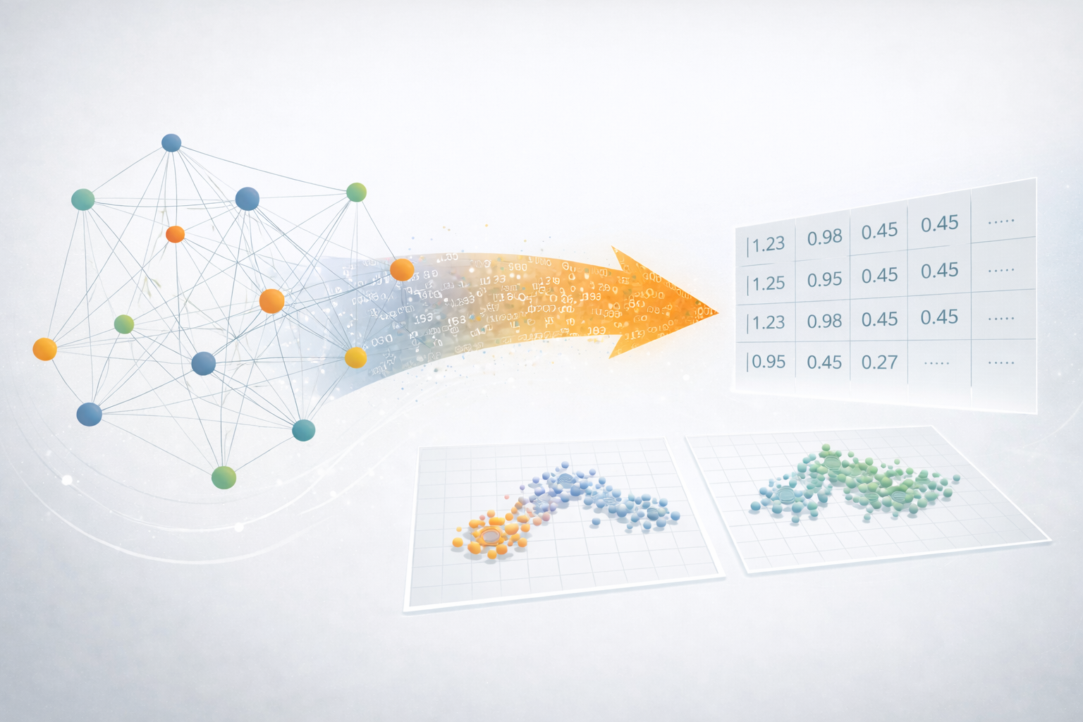
So ideally, we’d have a way to convert a graph into a matrix that a model can crunch through.

And actually, we already have one: the adjacency matrix. It’s a giant grid where each row and column represents a node, and each cell tells us whether—or how strongly—those two nodes are connected.

It’s a great first attempt at making graphs machine-friendly… until the graph gets big enough that the matrix balloons into the digital equivalent of a thousand-page spreadsheet. And that’s where embeddings begin to shine.

FastRP Under the Hood

Imagine you wanted to compare 1,000 people who filled out surveys about how much they liked 100 different media figures, resulting in each person having 100 dimensions of media-figure preference. It would be really time-consuming to compare each of these surveys to each other to see who had the most similar taste.

In fact, if you wanted to measure how similar these people are to each other, you’d need to compute distances between all 1,000 points in this 100D space—which gets computationally expensive.

Instead, we could represent the results as a matrix with 1,000 “rows” (one for each person) and 100 columns (one for each media figure). If you multiply this matrix by a randomly generated matrix with 100 rows and, say, 10 columns, you’ll end up with a new matrix that compresses each person’s data into just 10 numbers.

Even though this transformation uses random numbers, it’s the same random projection matrix applied to everyone—so the relationships between people are preserved. In fact, the relative distances between people stay mostly the same, even though we’ve reduced the number of dimensions. This is because the random fluctuations that you get when multiplying by a random number will tend to average out to zero when you multiply enough of them across all the dimensions.

In our example, we will be working with very small numbers. Our graph will look like what you see above!

Step 1: One-Hot to Random Projection

First, we need a simple way to convert each node in our graph into a number. One easy method is a one-hot vector. Since we only have three nodes, each one gets a short three-number list with a single 1 in its own spot, which can also be represented as a matrix.

This works, but it’s mostly zeros—so it’s not very compact or efficient. To shrink it, we multiply it by a random projection matrix, which is just a small table of random numbers.

Because we have three nodes, this matrix needs three rows. And since we want to reduce everything to two numbers per node, we use two columns:

After we multiply the two matrices, each node will be represented by just two numbers, capturing the same idea in a much smaller form.

So let’s start by looking at Node A, which corresponds to the first row in our matrix. Basically, we’re going to multiply the top row in H by each row in R (and add together all the values):

When we do that for each row, we get something like what you see below. You may notice something funny: this output is identical to the random projection matrix. That’s not a coincidence. Each row of the one-hot matrix has a single 1, meaning it simply “picks out” the corresponding row in the projection matrix. All the zeros wipe out everything else.

Because of this, FastRP doesn’t bother building one-hot matrices or doing this multiplication at all. It just assigns each node a random dense vector directly—the same result, without the extra steps.

However, this is exactly how the algorithm works conceptually, and it’s important to understand the logic before moving on to more complex steps, such as neighbor aggregation.

Step 2: One-Hop Neighborhood Aggregation

We can represent the connections from our earlier graph using something called an adjacency matrix, which shows which nodes are connected to which. Let’s look at our adjacency matrix:

In our matrix, a 1 means there’s an edge from the row node to the column node. Since our edges are directed, A -> B doesn’t imply B -> A.

We’ll use it to aggregate neighbor embeddings by multiplying it with the initial embeddings from Step 1.

Let’s start with Node A since it has the most outbound relationships. I’m going to write everything out to make this as clear as possible, even if it’s not the correct notation.

Which equals [-0.6, 1.0].

Remember, we multiply each column in [0,1,1] by its corresponding row in our matrix. That gives us the three vectors we need to add together to get our final embedding. Notice how this reduces three numbers down to two?

Next, let’s do Node B:

Because Node C has no outbound relationships, we will get all zeros for the final “row” in our resulting matrix found below.

So what exactly do we have here? We have a matrix where the first row represents the outbound relationships of Node A, the second row represents Node B, and the third row represents Node C.

Step 3: Reprojection and Weighted Sum

When we multiply our node vectors by the adjacency matrix, something subtle happens: many of the vectors start to look the same because they’re built from the same neighbors. It’s like taking three different colors of paint and mixing them with the same two new colors—pretty soon, everything turns into a similar shade.

Reprojection is our way of keeping the colors from blending into one muddy mix.

Basically, we are going to multiply our matrix by yet another random matrix to keep each vector for each node sufficiently distinct.

But how large should this new random matrix be? When multiplying matrices, the number of columns in the first matrix must match the number of rows in the second. So, our new random matrix must have 2 rows. If we want to keep the output in the same 2D space, we need a 2 × 2 random-projection matrix—like this:

We will then need to multiply this matrix by our resultant matrix from step 2. Doing so will yield us this:

This represents the embeddings for the one-hop neighborhood for each node. We can then combine this with our original set of embeddings, using a weighted sum. We will assign our first set of embeddings, which represent the original positions of the nodes, a weight of 1, and our second set of embeddings, which represent the direct neighbors, a weight of 0.8.

That will give us the following:

Node A:

Node B:

Node C:

And, voila! Now we have a set of refined embeddings that now encode not just each node’s identity, but also its immediate neighbors.

We could continue down this path by following the same steps, but instead of looking at one-hop neighbors, we could look at two-hop neighbors; however, at this point, it will be largely the same practice. In fact, the number of neighbors away is actually a parameter that you can tune.

Let’s get back to our original mission: to take something as complex as a graph and reduce it to fewer dimensions. Through random projections, we were able to assign a numeric value to each node’s position and further encode its neighbors’ positions.

Now, those compact representations let us treat nodes like any other feature vector, making them easy to plug into standard models such as classifiers, regressors, or clustering algorithms.