The definitive guide to building a predictive model in Python

AI Research Engineer, Neo4j
12 min read

Predictive modeling is one of the most fundamental tasks of a data scientist, and you’ll encounter it in nearly every job and industry in the field. Keeping your knowledge and skills up-to-date is essential to driving efficiencies and revenue at your company.
In this article, you’ll discover how to build a predictive model in Python, including the nuances of installing packages, reading data, and constructing the model step-by-step.
Predictive modeling fundamentals
Predictive modeling is the use of statistical models to make predictions about the future from past data. This practice can refer to both the development of models from mathematical principles and the application of those models to real-world data. Data scientists are generally only interested in doing the latter — using existing models to make predictions.
Some everyday uses of predictive modeling in industry include:
- Identifying content-violating posts for a social media site
- Trying to predict the future value of a stock in finance
- Estimating the likelihood that a policy gets claimed in insurance
- Predicting the effectiveness of an advertising campaign
Of course, these are just a few of the many ways you or your team may use predictive modeling to drive organizational efficiency.
Steps to build a predictive model
Before diving into the specifics of building a predictive model in Python, it’s critical to understand the primary steps for predictive modeling, regardless of what programming language you use. Here’s a look at these foundational actions.
1. Collect and organize the dataset
The first step to constructing a predictive model is to gather the data you want to build your model off of. Models need data so that they have a reference for how variables influence the outcome you’re trying to predict.
On the job, your company will likely provide a database made in software like MySQL, MongoDB, or Neo4j to query your data. But on your own, you can get data by downloading it from a website or scraping it from the web.
2. Clean the dataset
Often, a dataset won’t be “clean” when you first open it up. Some examples include:
- Different spellings for column values (i.e., having “Texas” and “TX” in a “state” column)
- Incorrect decimal points or units (i.e., price information in cents rather than dollars)
- Missing data (i.e. having values labeled as “NULL”, “NA”, or “NaN”)
Since there are infinite ways that someone may wrongly display data, there’s no “one size fits all” approach to resolve these issues. The optimal strategy is to think critically about addressing each problem independently. Some best practices are:
- Never process “numerical” data that are descriptive (i.e. zip codes) as an actual number.
- It’s generally better to drop missing data rather than replace it with zero or the average.
- Ensure there’s exactly one way to label a category (so nothing like “small” and “Small” and “S”).
3. Choose a methodology/algorithm
The next step is to choose the model you want to use to generate your predictions. There are hundreds of models to choose from, and one way to narrow them down is to determine if a regression or classification model suits the situation.
Regression models output a numerical estimation of the value of a specific variable, i.e. the price of a stock. Classification models output a statement of what “class” or “category” a data point belongs to, i.e. if someone defaults on a loan or not.
To choose between using a regression or classification model, ask yourself what you want the output to be. If the output is a number, go with a regression model. If it’s a category, go with a classification model.
As for what specific model to pick, feel free to review the sklearn user guide for high-level overviews about different models.
4. Build the model
The final step is to build and fine-tune the model. This step is the most straightforward because you can follow a standard format for training the model once the data is ready. It’s also easy to evaluate how well your model performs on the data you provide it.
Predictive modeling in Python
No matter what programming language you use, there will be language-specific packages, functions, and syntax you’ll need to use. Python is no different.
Data scientists can generally conduct predictive modeling in Python through the NumPy, pandas, and scikit-learn packages. Pandas and NumPy can help you load and manipulate data, while scikit-learn lets you build the predictive model. A more specialized model may use additional packages.
How to build a predictive model in Python
To show you how to perform predictive analysis using Python, we’ll use the example of predicting which lenders will default on their loans. This process boils down to three steps:
- Install and Import Python Libraries
- Explore, Organize, and Clean the Data
- Built and Evaluate the Model
Let’s get started.
1. Install and import Python packages
First, install the packages needed to load the data and create your model. Consider modeling in a Jupyter Notebook rather than a raw Python file so that you can easily see the output of your code.
Assuming that you already have Python and Jupyter installed, open Powershell (if on Windows) or Terminal (if on Mac or Linux) and type the following command:
pip install matplotlib numpy pandas scikit-learn
Then start up Jupyter Notebook with the command:
jupyter notebook
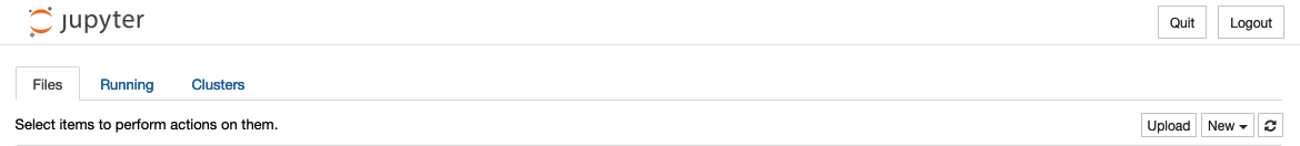
Click the “new” drop-down menu and choose “python” to create a new notebook to work in.
To import the packages, simply put these statements at the start of your notebook and run it.
import matplotlib.pyplot as plt
import pandas as pd
import numpy as np
2. Explore, clean, and organize the data
With the Python packages ready to go, it’s time to download the data so you can prepare it for modeling.
Download the dataset from Kaggle, unzip the archive.zip file, and drag the train_LZV4RXX.csv file to the directory you’re working in.
Now you’re ready to start exploring the data.
Read the dataset
To read the dataset into the notebook, you can use pandas’ `read_csv` function.
raw_data = pd.read_csv('train_LZV4RXX.csv',index_col='loan_id')
It’s good practice to store the unmodified data in a separate variable from the data you’ll be modifying, in case you make a mistake.
data = raw_data.copy(deep=True)
Explore the dataset
To display a DataFrame, you can append the variable name to the end of the cell and run the cell’s code.
data
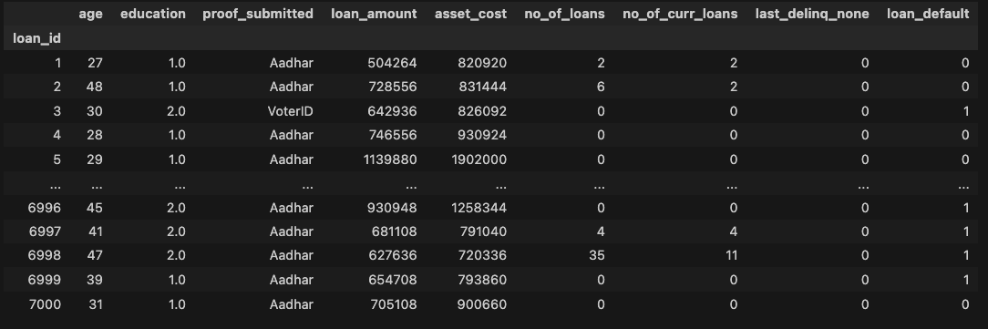
In this table, `loan_default` is the “target column”— the column you’re predicting using the other columns. `1` means that the borrower defaulted and `0` means that they paid back the loan in full.
Here, there are two situations you can investigate:
- The `education` column only has `1` and `2` as values, indicating that it might be a mislabeled categorical column.
- `proof_submitted` is a categorical field, so you’ll want to check that there are no misspellings or duplicate categories.
To get the values of only a specific column, you can index the data variable with the name of the column you want, like so:
data['proof_submitted']
loan_id
1       Aadhar
2       Aadhar
3       VoterID
4       Aadhar
5       Aadhar
        ...
6996    Aadhar
6997    Aadhar
6998    Aadhar
6999    Aadhar
7000    Aadhar
Name: proof_submitted, Length: 7000, dtype: object
Use the `unique` method to find unique values of a specific column.
data['proof_submitted'].unique()
array(['Aadhar', 'VoterID', 'Driving', 'PAN', 'Passport'], dtype=object)
data['education'].unique()
array([ 1.,  2., nan])
It seems there are no duplicates in the `proof_submitted` columns, but the `education` column has at least some missing values (represented by `nan`).
Normally, you might want to remove data points with missing values, but these instances demonstrate the need for careful consideration during exploratory data analysis. Since the only other values of `education` are `1` and `2`, you can assume that `nan` represents a “zero” class. So it would be something like `nan` is a high school dropout, `1` is a high school graduate, and `2` is a college graduate. Go ahead and modify this column to reflect these corrections before you feed the data into your model.
Now that you’ve addressed the categorical columns, let’s move on to the numerical columns. The easiest way to get a glance at numerical data is to plot a histogram:
data.drop(['education','loan_default'],axis=1).plot(kind="density",subplots=True, sharex=False, figsize=(30,30),xlim=0)
plt.show()
You can check the pandas documentation for what the arguments passed to `plot` do.
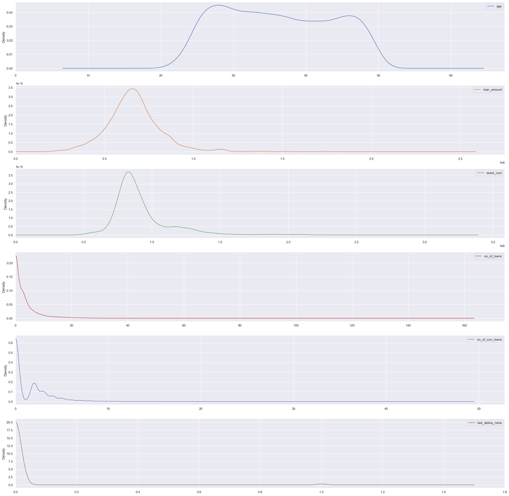
The density plots show that the distribution of all the variables is reasonable, so there’s no need to correct the scale or remove outliers. Note that `last_deliqn_none` is centered around zero and one because it’s a boolean column.
The final situation to check for is “class imbalance” which is when one class of the target column is overrepresented in the data.
data.groupby("loan_default").count()/len(data)
In this code cell:
- `groupby` organizes the data by the `loan_default` column
- `count` aggregates data by the number of instances in each class
- Division by `len(data)` makes the values display as percentages rather than the raw count
loan_default
False   0.6
True    0.4
Name: age, dtype: float64
There are more people that haven’t defaulted than have in the dataset. This disproportion is problematic because models created using this data will automatically be more biased toward predicting people who won’t default.
Luckily, it’s very easy to resolve this issue by specifying that the dataset is unbalanced when you go to create the model.
Clean the dataset
Now that you’ve investigated the data a bit and noted what to change, it’s time to clean and modify the data so that you can feed it into a model.
Start by fixing the `education` column. Create a function that assigns each of the values in the column (`1`,`2`, and `nan`) to a different category and apply it to the column, like so:
def get_education_category(education_value):
   if education_value == 1:
       return "Group_1"
   elif education_value == 2:
       return "Group_2"
   elif np.isnan(education_value):
       return "Group_3"


data["education"] = data["education"].apply(get_education_category)
Data manipulation
With the data now cleaned, the last thing to do is to manipulate the data so you can pass it into a model.
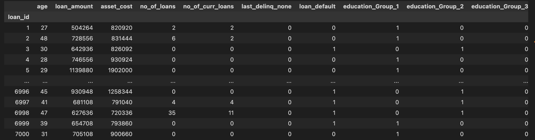
An important step in this phase is to make “dummy columns” for the two categorical columns — `education` and `proof_submitted` — since scikit-learn models can only read in numbers, not strings. The `get_dummies` function can quickly create the needed columns.
data = pd.get_dummies(data,columns=['education','proof_submitted'])
3. Data modeling
Now it’s finally time to model the data. For that, you’ll want to choose two tools:
- A model/algorithms to use
- A score function to use
Models are mathematical algorithms that essentially tell your computer how it should go about making predictions. A score function is a way of judging the performance of the model’s predictions.
To know what model to select, please reference the sklearn user guide for an overview of different models, as there are far too many to cover here. But, some points of comparison to consider when choosing a model include:
- Speed
- Explainability/Interpretability
- Tendency to overfit/underfit
Score functions differ in their priorities. They can prioritize minimizing false negatives, false positives, or a mixture of both. Determine if false positives or false negatives are more damaging in your specific case. For example, in healthcare, false negatives in disease diagnosis can be fatal while a false positive typically isn’t life-threatening. If you want to look at the various score functions available, Wikipedia’s “Confusion Matrix” article is a great resource.
Since the model will be predicting a boolean value (whether or not the borrower defaults), you’ll want to use a classification model. We’ll be picking a Random Forest model since it’s fast and robust to both underfitting and overfitting.
For the score function, assume the firm is risk-averse and wants to minimize false negatives (i.e., times when the model predicts a borrower won’t default and they do). The recall score function captures this goal; it’s defined as:

With the model and score function chosen, you can now start actually coding the model. First, split the data into “training” and “test” data using scikit-learn’s `train_test_split` function. It’s essential to do this because if you provided the model all of the data, it would just repeat the data verbatim for its predictions.
from sklearn.model_selection import train_test_split


X_train, X_test, y_train, y_test = train_test_split(
   data.drop(["loan_default"], axis=1),
   data["loan_default"],
   test_size=0.4,
)
The first argument provides the columns you’ll use as predictors (the “independent variables”). The second provides the target column. The `test_size` parameter determines how much of the data you’ll reserve for testing. Any value between `0.4` and `0.6` is considered good practice.
Next, import the model and score function.
from sklearn.ensemble import RandomForestClassifier
from sklearn.metrics import recall_score
Most models have “hyperparameters” you can adjust to make different variations of the model. The `GridSearchCV` class provides a way to test multiple sets of hyperparameters and pick the best ones.
from sklearn.model_selection import GridSearchCV


clf = GridSearchCV(
   RandomForestClassifier(),
   {
       "criterion": ["gini", "entropy"],
       "max_depth": [50 + i * 10 for i in range(10)],
       "oob_score": [True, False],
       "max_features": ["sqrt", None, 6],
       "min_impurity_decrease": [0.00, 0.001],
       "class_weight": ["balanced"],
   },
   scoring="recall",
   n_jobs=-1,
   verbose=3,
)
You can check scikit-learn documentation for a description of what these hyperparameters do. Note that `class_weight` is set to only be `”balanced”` since the target value wasn’t evenly split between the people who did or didn’t default.
clf.fit(X_train, y_train)

Fitting 5 folds for each of 240 candidates, totalling 1200 fits
[CV 2/5] END class_weight=balanced, criterion=gini, max_depth=50, max_features=sqrt, min_impurity_decrease=0.0, oob_score=False;, score=0.297 total time=   0.7s
[CV 3/5] END class_weight=balanced, criterion=gini, max_depth=50, max_features=sqrt, min_impurity_decrease=0.0, oob_score=False;, score=0.373 total time=   0.7s
[CV 1/5] END class_weight=balanced, criterion=gini, max_depth=50, max_features=sqrt, min_impurity_decrease=0.0, oob_score=False;, score=0.376 total time=   0.7s
[CV 5/5] END class_weight=balanced, criterion=gini, max_depth=50, max_features=sqrt, min_impurity_decrease=0.0, oob_score=True;, score=0.307 total time=   0.8s
…
To print the score and parameters of the best model found during the search, use:
print(
   "Recall score of best model:",
   round(recall_score(y_test, clf.predict(X_test)) * 100, 2),
   "%",
)
print("Best model parameters:")
clf.best_params_

Recall score of best model: 56.72 %
Best model parameters:
{'class_weight': 'balanced',
 'criterion': 'gini',
 'max_depth': 70,
 'max_features': 6,
 'min_impurity_decrease': 0.001,
 'oob_score': True}
Our recall score says that, of borrowers that ended up defaulting, the model correctly identified 56% of them, which is pretty good!
Get started with predictive modeling in Neo4j
In this article, you learned how to build a predictive model using a dataset from Kaggle. While this dataset was relatively clean from the start, in the real world, you’ll query data from a database, and even after you’ve done that, you’ll need to configure connections to the database in Python.
An analytics and machine learning engine like Neo4j’s Graph Data Science can help you query and configure data easily using the relationships in your data to improve predictions. It plugs into enterprise data ecosystems directly, so you can get more data science projects into production quickly and efficiently. Check out this other blog post to learn how to improve your machine learning model in Python using Neo4j Graph Data Science.
With its native Python client and intuitive Graph Data Science API, there’s no need for a lengthy setup to begin creating predictive models. This, combined with access to pre-configured graph algorithms and automated procedures, means your organization can start turning your organization’s data into actionable insights from Day 1.
Additionally, Neo4j Graph Data Science integrates directly with popular platforms like Apache Arrow, KNIME, and Dataiku, alongside providing automated MLOps services. It’s quick and easy way to reuse, share, and modify predictive models, so no matter your current tech stack, you can easily integrate Neo4j into your team’s workflow.
Get started with Neo4j Graph Data Science in Python today and improve your machine learning and predictive modeling capabilities.
Share Article


Explore
Related Articles
Neo4j Named “One to Watch” in Snowflake’s 2026 Modern Marketing Data Stack Report

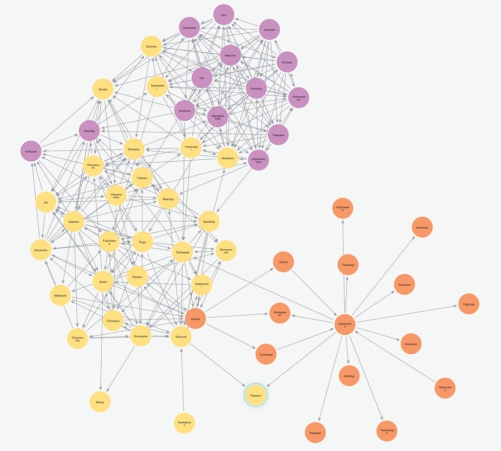
SumoDB in Neo4j: Chaining Multiple Graph Algorithms in Snowflake — Part 3


Why machines need embeddings: Turning graph structure into features