Building Spatial Search Algorithms for Neo4j

Editor’s Note: This presentation was given by Craig Taverner at NODES 2019.

Presentation Summary

Craig Taverner, Senior Software Engineer at Neo4j, presents Building Spatial Search Algorithms at Nodes 2019.

Taverner briefly runs over some Neo4j history before presenting the two new data types debuted in Neo4 3.4: temporal and spatial. For the sake of this presentation, the focus will be on spatial graph data.

In the Spring and Summer of 2019, Eindhoven University student Stef van der Linde interned at the Neo4j office in Malmo and did some work on Spatial Algorithms.

The task he was given was to develop a few sample complex algorithms. Some of the conclusions were that some data models were a lot faster than others. Speed makes a huge difference when you are considering which data model you choose to use and how you are able to write complicated algorithms within it.

An example would be a polygon with holes that have polygons inside them, you need to have a complicated data structure for that.

There are a lot of valuable features in this program like route finding using Shortest Path, Dijkstra’s algorithm and A Star.

There is also point-in-polygon which has the ability to limit destinations to certain regions.

Polygon area is how we calculate areas. Using the four algorithms that Taverner demonstrates, we are able to calculate the areas, intersection, distances and convex hulls of a polygon.

Polygon intersection, though a little bit complicated, is not too difficult. When you break down all of the geometries into pieces of line segments that don’t overlap, you end up with a monotone chain sweep line. When you sweep across this line you will reorder the points and detect the intersections. At the end if you have no intersections you now know that they don’t intersect. If you do have intersections, you are able to produce an intersection geometry.

Polygon distance uses the doubly nested loop to consider all combinations, and then finally get down to what is the distance between two points. We are also able to use Cypher to query this.

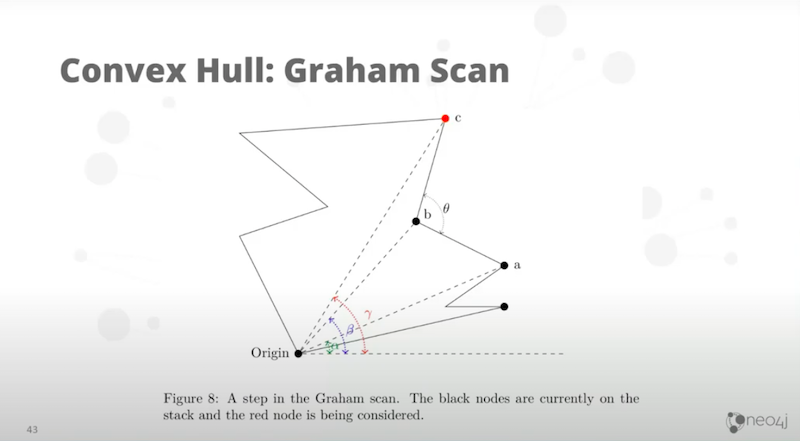
Finally, convex hulls are like taking a rubber band around a shape, the elastic is not going to dent in. Instead, it is going to dramatically simplify the shape of the polygon. The first thing you do with a convex hull is turn it into a bag of points then pick an origin. When comparing any three consecutive points, in this case A, B, and C, we calculate the angle from A to B versus B to C. If the angle at B. If it’s less than 180 degrees, B is a concave piece and we throw it away. This algorithm throws away all the points that create anything concave and reduces the total number of points dramatically. Then it will go A, C, to the next one and do the angle there. It’s going to sweep all the way around and throw away all the concave points.

Full Presentation

Hello. My name is Craig Taverner and I’m going to be presenting Building Spatial Search Algorithms for Neo4j.




This is going to be based on a mixture of some old work that we’ve done as well as something we did very recently this year.

I”ll start with the old stuff and break it down into a summary. Then, I’m going to talk about what’s currently available in the standard Neo4j. Finally, we will move onto the spatial algorithms themselves.

We’ve done some recent work in an internship where we built some new algorithms. I’d like to show you how we demo those in a full stack application.

History

I’ve been involved in Neo4j since 2009. In 2010, I did collaborative work.



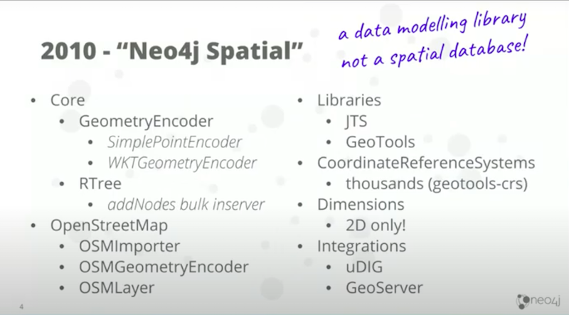
I was a community member at the time. Before I worked for Neo4j, I did a collaborative project with them to build a GIS modeling library which we called Neo4j Spatial.

This is not something we recommend you use these days because it was designed for the embedded deployment that Neo4j used to focus on. Now Neo4j has been a server deployment for many, many years.

You are able to access some of this through the server, however, its history shows. It’s not a spatial database. It’s a spatial modeling library. It’s strength is that it wraps well-known libraries like JTS and GeoTools and is very comprehensive.

The server is not very scalable and it has issues that you would experience in an enterprise deployment where you have high concurrency, high volume situations. I’d only look at this if you are interested in the features and you’re not going for high concurrency, high volume.

One thing I wanted to highlight is that in 2010, we all wrote an OpenStreetMap importer and an in-graph OpenStreetMap model. This is something that we still use today and is a major part of the algorithm work that we have done this year.

I drew this in 2010 when we first built OpenStreetMap.



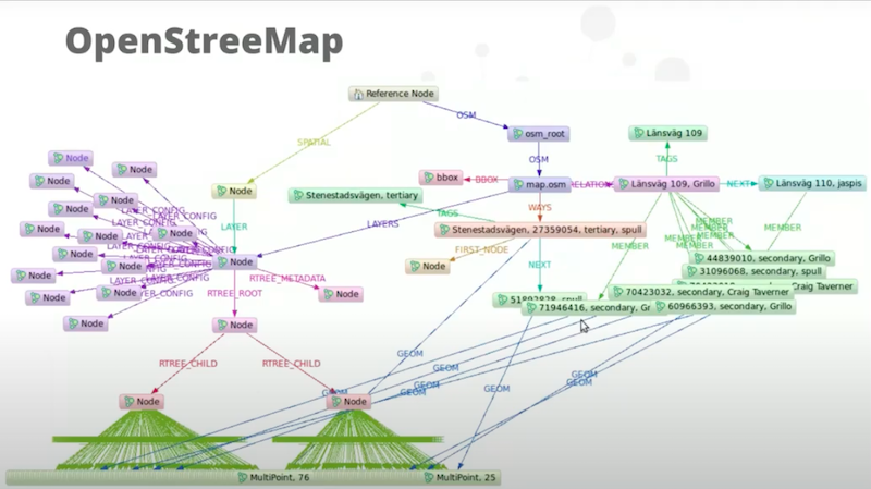
It’s a bit archaic but the model itself is still very similar. The most interesting thing to take away from this is that OpenStreetMap is one single, fully connected graph of the planet, and that’s fantastic! There is almost nothing in GIS that’s like that.

The last thing to say about the old library is it’s very extensive but only if you use it in embedded mode because it wraps all of these other capabilities.



In 2016, we supported our servers by adding procedures that allow users to access a reasonable subset of its capabilities within a server deployment.



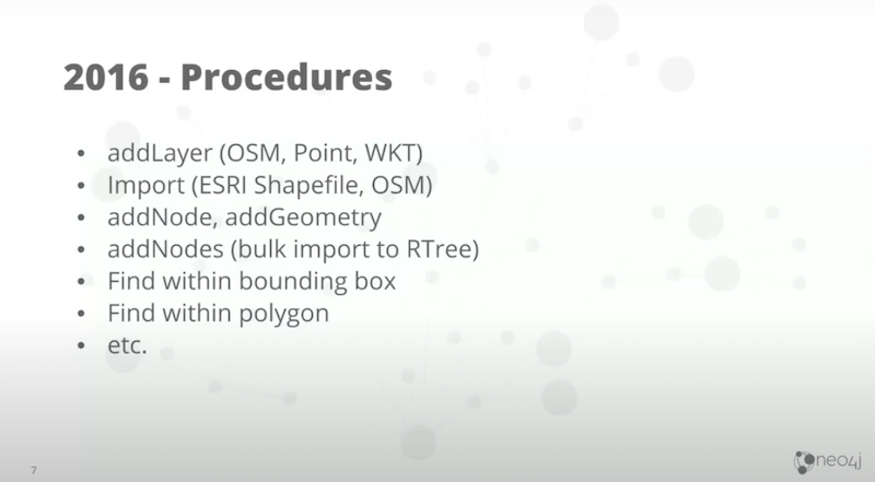
That’s the last thing to say about the old library because I’m assuming 99% of you are going to work with the new stuff. It’s good to know the old one’s there in case you need to use some of that.

In that case, what is new?

Neo4j. 3.4

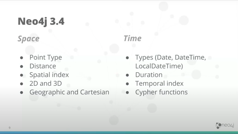
Neo4j 3.4 introduced two new data types.



This is the first time in a decade that Neo4j had introduced a core data type that was new.

The one was the temporal types of which there were a whole bunch. There’s lots of documentation on that here.

Next, there were the spatial types. We only supported spatial types natively in the graph one type and that’s a simple point. We did make it a little bit powerful in the sense that you are able to have both 2D and 3D points. Both points could be in geographic and Cartesian coordinate systems. I’ll talk more about geographic and Cartesian throughout this presentation because it’s an important factor when it comes to algorithm development.

As for 2D and 3D, this presentation is going to be about 2D only.

Another thing about the native type is that we developed a spatial index. There’s only one algorithm built into Neo4j and it’s distance. I say only one but there are actually two incarnations of it, one for Cartesian, one for geographic. These have slightly different calculations because Cartesian is just Pythagoras. Everyone has written Pythagoras, whereas geographic is a little bit more complicated with trigonometry.

Let’s briefly describe how the index works.



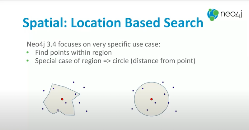
We targeted a particular use case which was to find points inside regions. Unfortunately, what’s built into Neo4j today only supports the special case of the region being a circle. This requires that you find points within the distance of a point of interest.

I will describe that now and then I’ll show you how you are able to enhance this to actually support regions, even if Neo4j doesn’t do it natively.

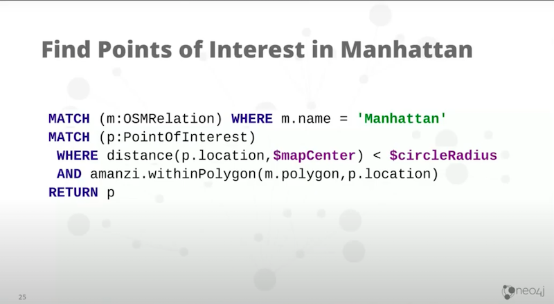
Say you have a query like the one below.



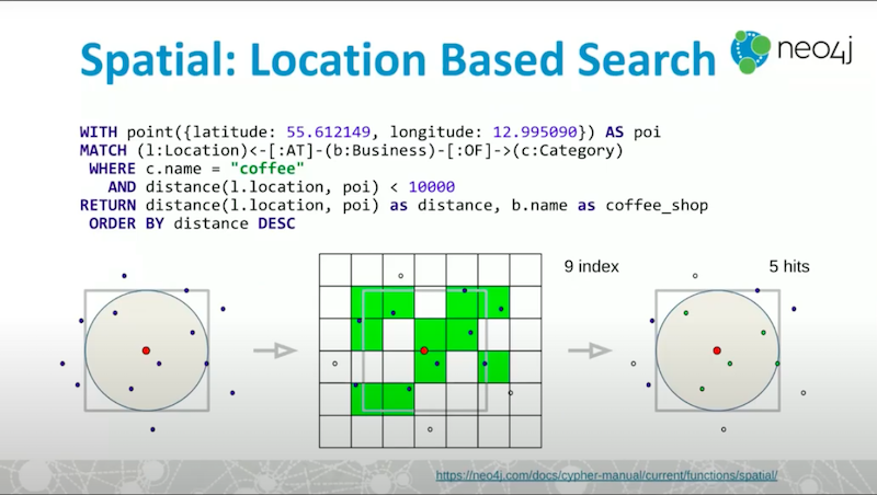
You’ve got some point of interest. It could be written into the query as I’ve done there or pass it in as a parameter, which is what we usually do in an application. Let’s say you have a graph that has businesses of a certain category and there are certain locations as expressed by the match expression up there.

You could have quite complicated queries that actually have predicates both on the category and the location and Cypher if there are indexes on both category and location. It will pick the most appropriate index for highest performance and return the results. The way it does it is with a spatial index, it identifies that distance function.

If you look at the predicate there after and it says the distance between the location of the business and the point of interest is less than 10 kilometers. It is able to realize that it could interpret this as an index query. It does that by putting a minimum bounding rectangle around that circle. It passes that into the index. That will return all the tiles that have points in that part of the rectangle.

Then we do a post filter. In this particular example, there were nine candidates filtered down to five.

You could imagine, even though we do a second pass filter, if you had nine million points, the index returning five million is giving you a massive performance advantage. We benchmarked this and it works very well, comparable to other spatial databases.

The last thing to say about the built-in support is what I said before about 2D and 3D. However, this time it’s about Cartesian and geographic.



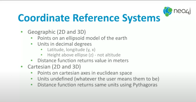
Some key points about geograpic are that the points are on an ellipsoid model of the Earth and they’re in decimal-degrees angles, latitude, longitude. This all means that the distance function is going to work differently.

In Cartesian, you have no units. Whatever the units are of your points will be the units of your distance. In geographic, we assume the locations are in degrees, decimal degrees, and will return distance in meters. Cartesian is very strict about what the units mean.

Spatial Algorithms

Let’s get on to an introduction to these spatial algorithms.



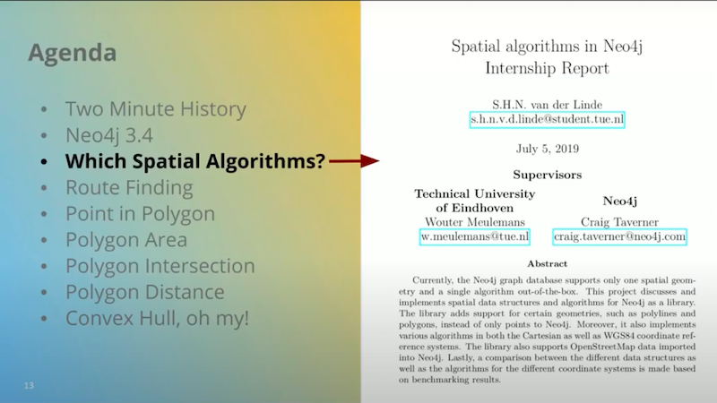
One of the motivations I have for giving this talk was that in the spring and summer of 2019, we had a very interesting internship as a collaboration between Neo4j and Eindhoven University. They had a student, Stef van der Linde who came out to Malmo and sat with us for three months and did some work on spatial algorithms.

The task that I set him was to develop a few sample complex algorithms. We didn’t go for coverage. We wanted to have a few complex algorithms that could be useful for benchmarking the performance of the algorithms in both Cartesian and geographic systems. A very interesting element of the work was to have the algorithms run on alternative data models. You could have a data model that is a polygon in the graph. Or you could have a data model that’s an array of points. You could have various different data models. We wanted to see how these algorithms would perform when comparing those.

Some of the conclusions were that some data models were a lot faster than others. That definitely makes a big difference to the data model that you plan to choose and how you’re going to model your data if you intend to write complicated algorithms on it.

Another key element for the geographic side is that we wanted this to work on OpenStreetMap data because that is such a valuable data source.

If you remember that really cluttered diagram I showed you a few slides before, Steph has redrawn it symbolically here, which is a lot easier to understand.



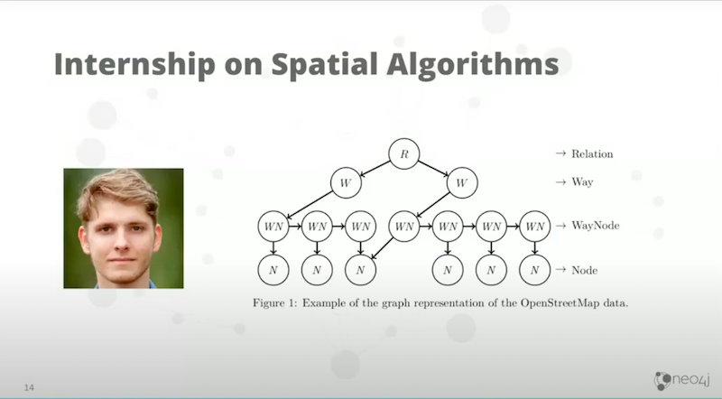
This is the typical tree structure of how you assemble complex geometries in OpenStreetMap.

The bottom row of that tree structure are the nodes. That word node is not a Neo4j node. That’s an OpenStreetMap node. The term means a point, a location.

Then, if you go to rows upwards, ways chain nodes together into a line segment. This is a chain of nodes which will represent a piece of the street or a border of the building or maybe a piece of the outline of an area of a park, of a province, administrative region, something like that.

It turns out that there’s an ability in OpenStreetMap to arbitrarily collect things together in progressively more complicated structures. That’s the relation concept at the top. Relation contains multiple ways, nodes and other relations and allows you to get a very complicated data structure.

An example would be a polygon with holes that have polygons inside them, you need to have quite a complicated data structure for that.

Steph modeled a few ways of doing this. This is the way that seemed to work best for us, if you take this example below, that’s a complex multi polygon.



Let’s say, there might be a game reserve or a native area or some kind of park that’s made of multiple disjoint areas and some of them have got lakes in them. In some of those lakes you have islands. Then, you end up with something quite complicated. We modeled it like you see on a tree structure like on the right. There, each simple polygon is a single node containing an array of points.

Now, Neo4j natively supports both point and arrays of points, just like it supports integer, array of integer and arrays of any other primitive types. That rule is very convenient. It means we could use the native Neo4j types in order to structure this. The complexity comes only in the tree structure which is working very well.

The demo I’m going to show today is based on this data structure. You are able to have multiple simple polygons containing multiple holes. These holes could contain multiple simple polygons, which could contain multiple holes, et cetera.

The data structure could be arbitrarily deep. This is possible in most GIS systems as well. It’s very convenient in a graph because we have the Vol/Length concept, the traversal of the graph to find these things.

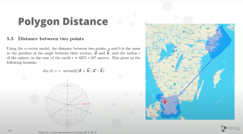
I mentioned before that geographic is a bit different from Cartesian. What Steph found is that there’s a whole class of maps for the spatial algebra that uses the n vector representation. A point on the surface of the planet is modeled by a vector normal to the surface, then two points, which make a great circle as you see on the right hand side below.



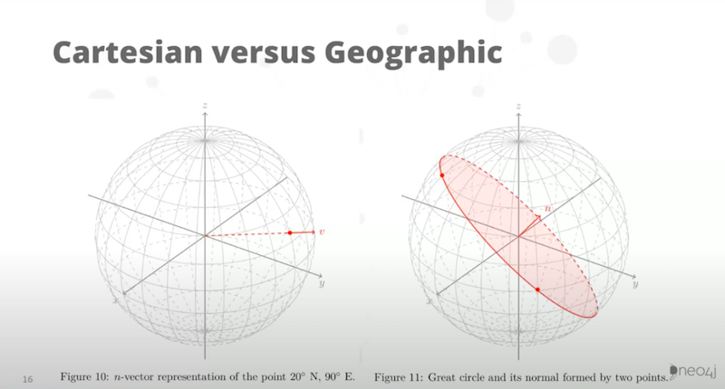
Cartesian and geographic are modeled by the vector normal to the great circle, which was shown above.

There’s quite a lot of algebra that we’ve got inside our algorithms that are based on this concept. I’m going to show you a little bit of that, but try to avoid going into too much detail because it’s a bit mathematical. It’s worth reading Steph’s paper if you want to know the details.

Route Finding

I have six algorithms to show you.

The first two algorithms were demoed last year at GraphConnect and in a few meet ups after that. After the first demo, we focused on the route finding and finding points in polygon.

Last year we went over simple route finding using Cypher for the built-in Cypher shortestPath function.



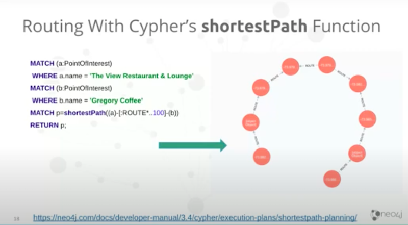
Shortestpath is not the best choice. It tends to give you a non-ideal path in the real world, that’s a limitation of using shortestPath.

Instead, what you want to do when traversing a path, is to have weighted relationships for at least the distance. You could use the time it takes to traverse based on speed limit and other things like that. In our demo, we used distance and it gave a much better approximation than shortestPath.



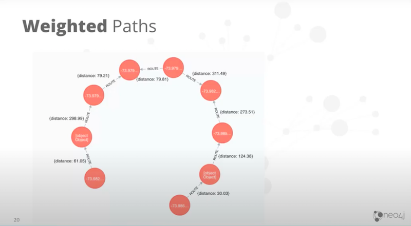
How do you do a shortestPath including a weighted function?

Cypher doesn’t have a method built-in, but Neo4j has had an embedded API since 2007. Luckily for us, the Epoch Library of Procedures has exposed that for us and that gives us access to these two algorithms.



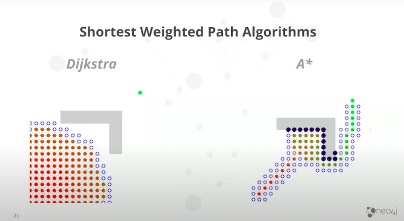
That is the Dijkstra’s algorithm, which considers weights. As such, Dijkstra will always find the shortest path based on weights. However, it doesn’t go very fast because it’s searching in all directions. It starts from one side and just searches in all directions until it finally finds the other node.

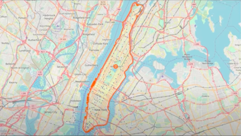
The A Star is a bit more clever. You give it two functions, one for the weights and the other one for a preferred direction Or it’s an additional cross-function, which in our case implies a preferred direction. A Star tends to be much faster. We demoed this last year in Manhattan. You could find the shortest part between where you were and the coffee shop that you wanted to go to and it worked very well.

Here’s a small animated GIF that Will put together showing you some of these shortest path calculations. It was quite effective.

Point in Polygon

The other thing we demoed last year was the point in polygon.

In the demo, I wanted to limit the potential candidate destinations to certain regions. I pre-calculated in the OpenStreetMap model the polygon of Manhattan, Brooklyn,Queens and other various areas. Next, I stored them as simple polygons.



In last year’s demo, we could only support simple polygons. Steph’s new stuff stores complex polygons and it’s a lot richer. I’m going to focus on the pointing polygon function.



I implemented the function in a very simple way. I’ve exposed it with this function, amanzi.withinPolygon. That’s a defunct library now because Steph’s project has completely rewritten all of this in a much better way.

What did my old library do? This is the point-in-polygon algorithm that I implemented.



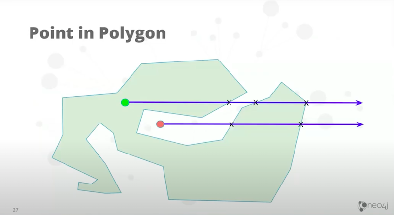
Take an array in any direction from the point of interest and count how many times it crosses a line and segment representing part of the polygon. If the number is odd, you’re with the polygon. If it’s even, you’re not. This works great in demos. However, there are some limitations. Point-in-polygon has some issues with geographic. There’s some possibilities where you might actually miss an intersection in some extreme cases because of the great circle curvatures. Also, it goes mad if you go near the Dateline or the Poles. Steph’s improved this a lot in the latest version.

One other thing I wanted to mention about this is in query.



I’m doing both a distance and a point in polygon. That’s because the distance triggers the index and the withinPolygon does not.

How do you trigger the index for polygons when Neo4j doesn’t know where they are? It’s possible to do it with another trick. That is if you have a second function called boundingBox.

Boundingbox takes the polygon and builds a rectangle around it, then you use the query. If you look at the third to last line, find the location that is greater than the bottom left corner, and smaller than that top right corner.

If you say that and write that to Cypher, it will figure out that you want to use an index and it will use an index. That’s a good way to trick Cypher into using index for a case where you wouldn’t think it’s actually capable. This is something that’s worth doing when you have larger amounts of data.

Before moving on to the next set of four algorithms that Steph implemented, I’m going to switch to a live demo.

This demo is the same application we used last year.




The demo has routing and all the rest.

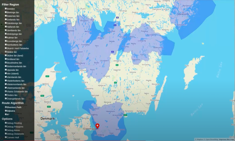
We are looking at Malmo. I’ll put this pin at the Neo4j engineering office.

I want to show you the new stuff and the new stuff involves the fact that we’ve built these polygons according to that tree structure I showed you. I select the polygon representing Scania.



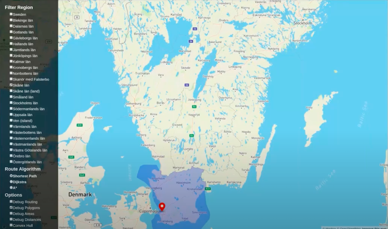
That’s the province that we have our office in. You’ll notice that the OpenStreetMap view of that province actually includes part of the sea because it’s part of the administrative region.

You could perform intersection calculations. I’ve done that in advance to show you the intersection between the province of Scania and the land area.

When I click on the map, I get the administrative region around Stockholm.



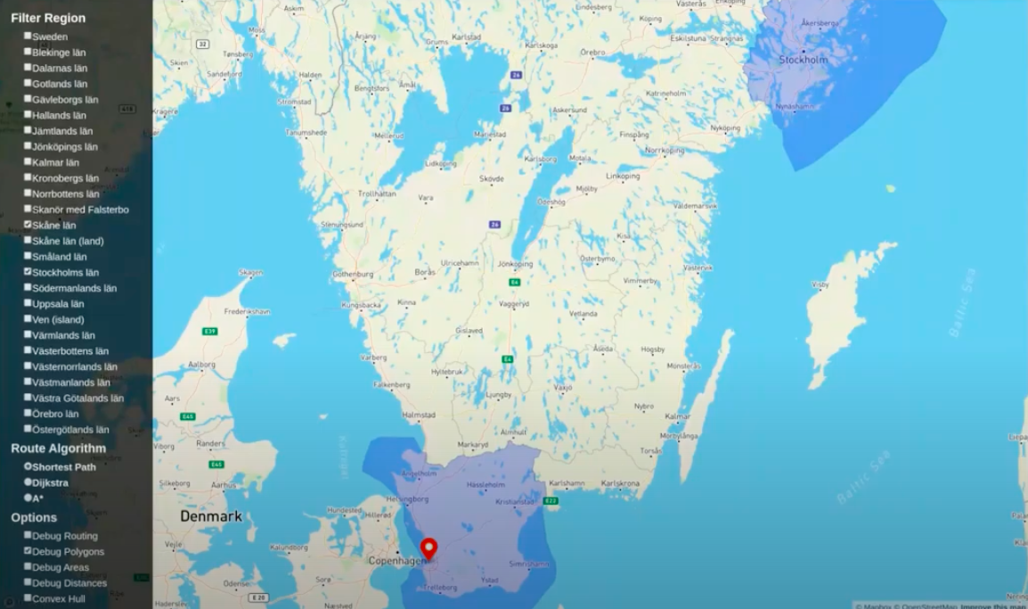
This uses the new version of the point-in-polygon function.



You are now able to show areas.



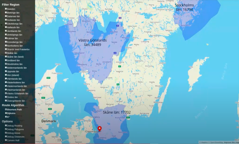
When I click to do so, I’m given the area of the polygon. That involves a traversal of the database, finding those calculating the area and returning it to the client. Additionally, it works very fast, which is nice.

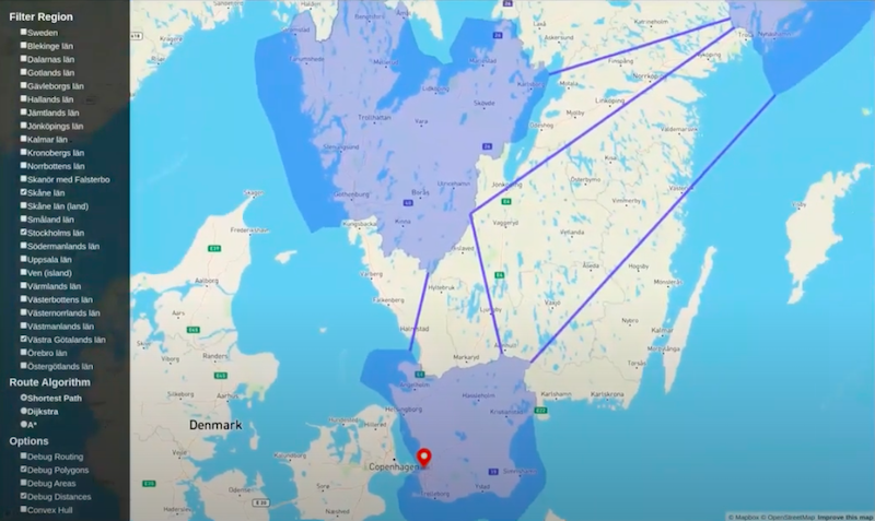
The next part of the demo is not fast. I am going to debug distances and ask it to calculate the distances.



That calculation takes a little while. I’m going to make it take even longer. I’m going to click on another polygon and this is going to add to that time.

While the system is busy calculating, I’m going to explain why it’s slow. The actual calculation between two points is very fast. The problem is finding which two points of the polygon are closest together. At the moment, we have an algorithm that is just brute force. It’s breaking up each of the polygons into little line segments and looking at all combinations.

Let’s compare Scania to Stockholm. Let’s say Scania is a thousand line segments and Stockholm is another thousand line segments. It’s going to look at a million possible combinations, calculate all those distances and then find the shortest before it’s going to return something. If you have three polygons, it’s going to do that three times over to find all of the combinations. It turns out that this one’s even slower than the last. This is because of something surprising which you will see when the results come in.



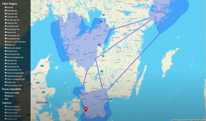
You would have expected one line between each of these provinces. However, look at this weird line in the middle here. When I first saw it, I thought I had a bug in my calculation. It’s not a bug.

This is actually a result of the way I queried the database. I’ll show you the Cypher query in the slides. It turns out this polygon has a hole.



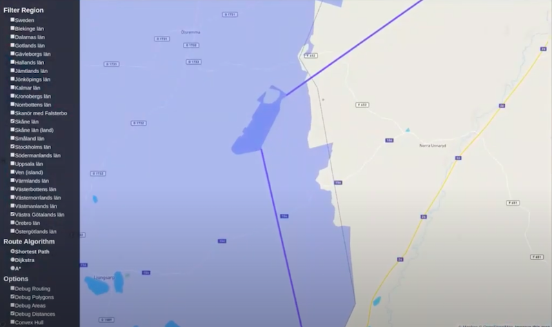
For some reason, the people living in this area wanted to be in the province adjacent to this area. They didn’t want to be in that province. This hole actually belongs to the other province. When I searched for my simple polygons to calculate distance, I searched for shells and holes. As a result, I’m finding the distances between four simple polygons here.



The last thing to show is the convex hull.

You’ll see that it’s very quick to calculate convex hulls. This was actually calculated live. I’m going to select a bunch of provinces.



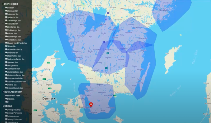
If I take away the convex hull, the provinces don’t overlap.

Polygon Area

You might already have guessed what a convex hull is. Let’s go back to the slides and I will explain in more detail.

We’re going to go through the four algorithms I just demonstrated. The calculation of areas, intersections, distances, and last but not least, convex hulls.

How do we calculate areas?



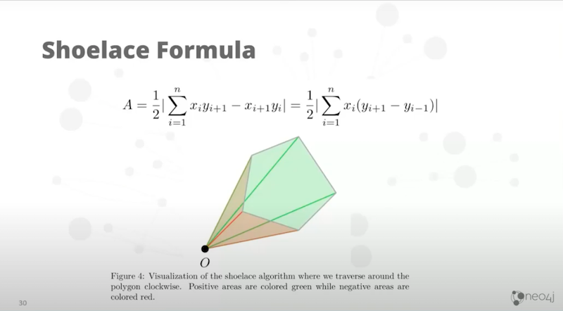
That equation might look a little scary, but it’s not.

The important points to notice is that you divide the area by half.

Then you sum over this xy. Your xy is the cross-product of two vectors.

Next, we subtract a different set of xys. To explain how that all works, look at the diagram.

Next, using the shoelace formula we choose an arbitrary origin. It doesn’t matter where. The origin could be inside or outside the polygon. In this case, we have it outside.

Now, you take each line segment that builds up the polygon. A line segment is made of two points. Calculate the triangle of those two points back to the origin. The area of that triangle is the cross-product of vectors, which gives you the area of a parallelogram.

You divide it by two and get the area of the triangle.

The division by two is coming from the conversion of the area of the parallelogram to the triangle.

All of the green triangles are the ones on the left. They are too large in area. You need to subtract these other orange ones. We need to know when we’re going around the polygon which side we are at. It actually works out naturally from the cross-product whether you’re going to get a positive or a negative value.

You take all the green and you subtract all the orange and bang, you have the area.

The shoelace formula is very fast and efficient. This doesn’t really work in geographic coordinates properly. There are some conceptual similarities. But in a geographic one, we do something that’s somewhat more complicated and involves calculating great circles.

Finally, there’s another theorem called Girard’s Theorem.



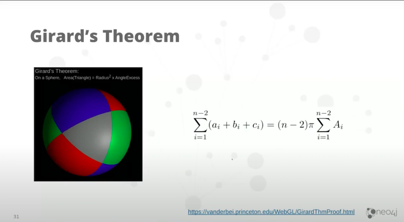
Girard’s Theorem produces the area as an equation from the great circles.

How do we query that?



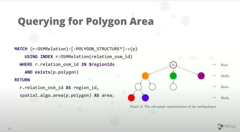
This top line in the match, you might have seen before. We find the top of the relation, then traverse down the tree structure of the subpolygons that are within that relation.

I do this for every single relation in my set of relation IDs. If I’m calculating the area for 20 polygons, then that will have 20 region IDs. The most important thing is the very last line. Return spatial.algo.area.

This function is taking the simple polygon, represented by that property or that node, passing it into the function and returning the area. As you saw in the demo, this is super fast, which is really nice.



While we’re showing one algorithm, I’m actually going to switch to the code for that.

How do you write code that is able to be accessed from Cypher like that?

Use this annotation.

“Spatial.algo.area” is the name that we refer to in Cypher. Then, we pass the annotation in the simple polygon as a list of native Neo4j points. We’re going to convert the annotation into the data structure that we’ve used in our library as a simple polygon.

This getCalculator says give me a calculator for Cartesian or geographic. It has a look at the data and then deduces that for you.

Now, we are able to go to the implementation of the function. The function is abstract because we have two different versions, Cartesian and geographic. Let’s go to geographic. It’s more complex but it’s not that bad.

It takes only one page to do Girard’s Theorem.



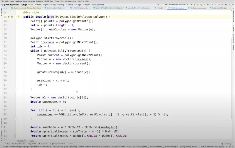
It’s as we said before, you’ve got to traverse to find all of the all of the great circles. Then you do this angular calculation that was in the equation that’s used by Girard’s Theorem, it works really well.

The other functions we have are spatial distance and we have spatial distance ends. The difference between these two is that in the spatial distance ends I’m going to return the distance as well as the two points representing which two points were closest between the two polygons that I showed earlier.



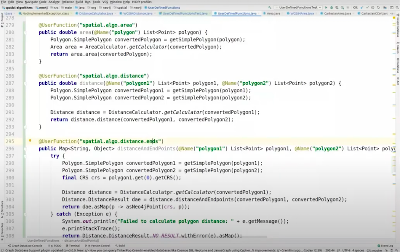
I wrote this function for the purpose of this demo.

Polygon Intersection

Intersection, it’s a little bit complicated. We’ve got this concept of a monotone chain sweep line.

Basically, you break all the geometries down into pieces of line segments that don’t overlap, or fall back on themselves on the x-axis. Afterwards, you will end up with this.



Then, you sweep across it. You sweep by reordering the points and then detecting the intersections.

Every intersection is added to a stack and you continue to sweep. At the end if you have no intersections, they don’t intersect. If you have intersections, you are able to produce an intersection geometry.

In geographic coordinate systems, we need to consider the fact that any two points don’t define only one possible line. They define a great circle. We could mean the other side. Which side do we mean? We’ve had to have some rules for deciding how that works. If you look at the intersections below.



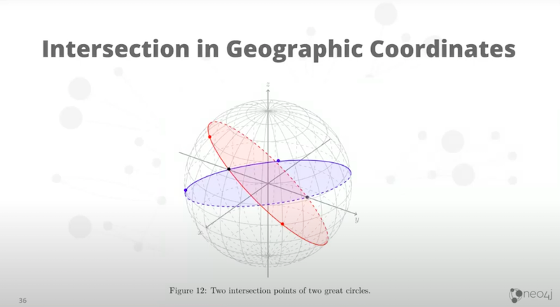
The red is defined by two red points. The blue is defined by two blue points. But which do we want? We don’t want the gray intersection. We want the black one and we need rules for defining that.

Another consideration for geographic is if the polygon touches or overlaps a pole, things go haywire.



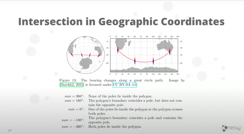
We have to have some detection code for that. It turns out that if you simply traverse around the polygon calculating the bearings and summing them all up, you will end up with 360 degrees.

If you don’t touch or overlap a pole, you will end up with plus or minus 360 degrees. This depends on whether the polygon is anticlockwise or clockwise, which is very important. Many GIS systems will use the direction to define whether it’s a shell or a hole, it’s quite important to know that. This all affects our area calculation.

Polygon Distance

The next topic is distance. The reason I did distance after the intersection is because the first thing the distance calculation must do is work out if they intersect and return zero. We have to code that intersection first.

We use the doubly nested loop to consider all combinations, and then finally get down to what is the distance between two points.

Below, I’m showing the version of the geographic coordinates, which is a cross-product again.



The arc converts it back into distance on the arc. This is a pretty straightforward equation. It’s very efficient and very quick. That part’s quick. The doubly nested loop is not as quick.

How do we query this? I’m going to show you Cypher examples for every one. This is the most complex Cypher.



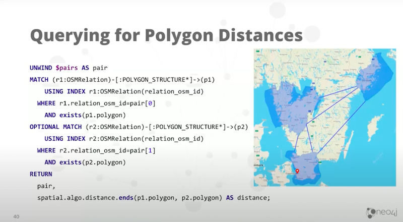
The part you most care about is the very last line. It reads, spatial.algo.distance.ends. If you want those points, pass in two simple polygons. All the rest of that Cypher is just finding all the polygons for those provinces. We need to make sure that we get the polygons and then we are able to pass the numbers into the equation.

What you might notice is that I’ve got this concept of pairs. I am passing into the query all combinations of provinces up front. I’m doing that in the application. Using just an integer ID we are able to do a quick search.

The first part of this query’s very fast. The only part that’s expensive is finding the closest points. I’d love to find a way to optimize that.

Convex Hull, Oh My!

The last thing to show you is the convex hull. You might have deduced what convex hull means by looking at this.



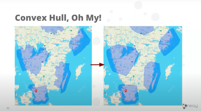
If you compare those two, the first thing you are able to see is that the right hand side looks much simpler.

However, the word convex means it doesn’t have any dents in it. It only has rounded surfaces. A dent is called concave, the polygons on the left have got lots of little dents. They’ve got convex and concave shapes to them.

A convex hull is like taking an elastic band around that shape, the elastic is not going to dent in. It all simplifies the polygon dramatically. First, we calculate this by knowing that convex hulls don’t require polygons. This could work with any kinds of geometries. You could have a complicated line segment, a highway or something, and you are able to make a convex hull around it. It’ll be the elastic band around all the points of that line segment.

The first thing you do is just turn it into a bag of points.



Then we pick an origin. Normally we pick an origin by convention, I pick the southernmost. If there are multiple ones at the same south latitude, you’re going to take the westernmost of those, the most negative or smallest X value and then you make that the origin.

Sort all other points in anti-clockwise order by angle. Then, start sweeping through it. The final product is the Cartesian version. I’ll show you the geographic version in a second. It’s only slightly different.

When comparing any three consecutive points, in this case A, B, and C, we calculate the angle from A to B versus B to C. If the angle at B. If it’s less than 180 degrees, B is a concave piece and we throw it away. This algorithm throws away all the points that create anything concave and reduces the total number of points dramatically.

Then it will go A, C, to the next one and do the angle there. It’s going to sweep all the way around and throw away all the concave points.

Why does this not work in geographic coordinates? This has to do with the angle and the lines because the calculation of an angle on a curved surface is a problem. What we really want to know is if you imagine a straight line between A and C, is B to the left or right of that line?

Another way of asking that question is the vector from origin to B, does it intersect? Does that line segment origin to B intersect the line segment A, C?



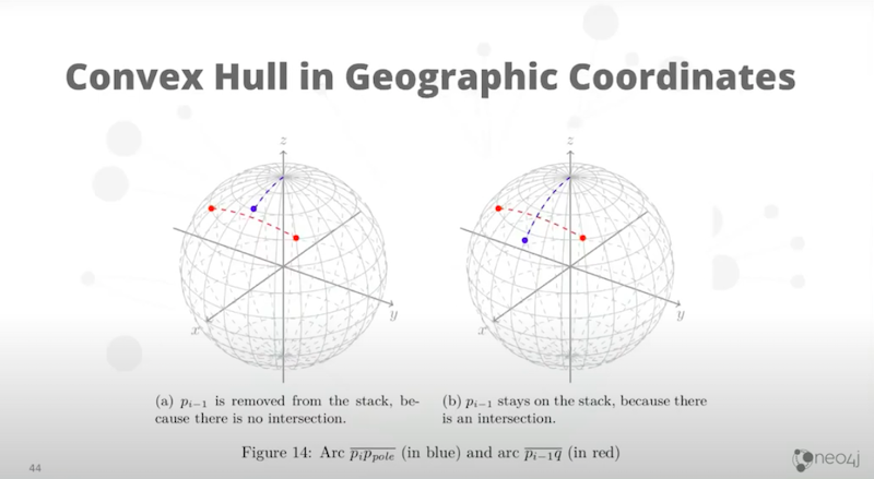
Here is the calculation.

You’ll notice that if you look at that red line, the line of constant latitude is a gray curve below the red line. We have to be aware of geographic coordinates. Otherwise, we’re going to get the calculation wrong. The actual line we care about is the great circle, which is the red line. We need to work out an intersection of the great circles. That’s the important part, and we’ve got that solved in other places. That gives us the convex hull in geographic coordinates.Instead of returning the polygon, we return the convex hull of the polygon super fast. It’s doing the calculation incredibly quickly.