In Microsoft Fabric, OneLake tables serve as the single source of truth – the foundation that keeps teams aligned and data consistent across the organization. That’s what breaks down silos and ensures trust in every insight.

So how does Neo4j graph intelligence fit in? In this walkthrough, we’ll start with OneLake tables, transform them into a connected graph, run graph algorithms to uncover scores and relationships, then write the enriched results back to OneLake.

Building a Better Retail Recommendation

What makes a good recommendation? Consider the humble grocery store coupon. Whenever I check out at the grocery store, if I scan my club card, there is a little machine that spits out a coupon, personalized for me.

This is a recommendation. But how does the store know what to recommend to me?

We’re going to learn how to make better recommendations from your OneLake data using Neo4j Graph Intelligence for Microsoft Fabric. 

Creating an AuraDB Instance

Our starting point will be OneLake tables, so if you want to follow along, load in the CSVs as OneLake tables in a lakehouse called “recommendations.” We’ll use them later.

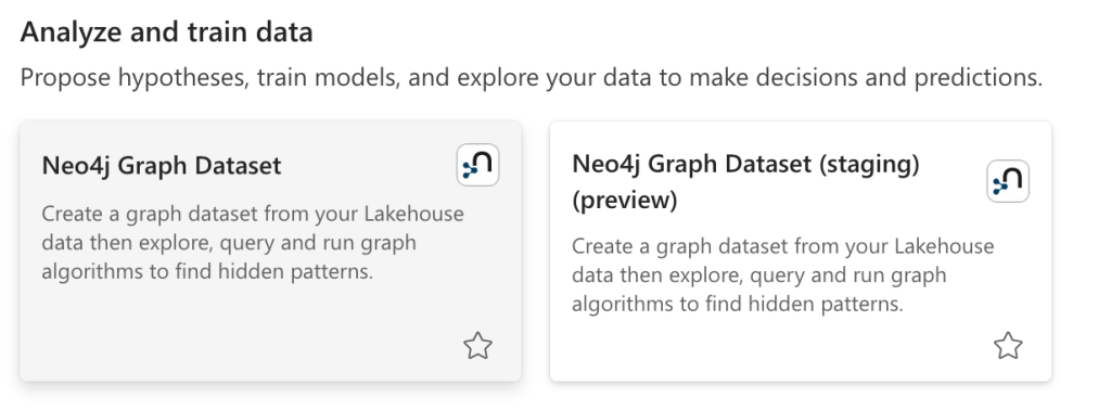
Start by creating a new item in your workspace and choosing Neo4j Graph Dataset.

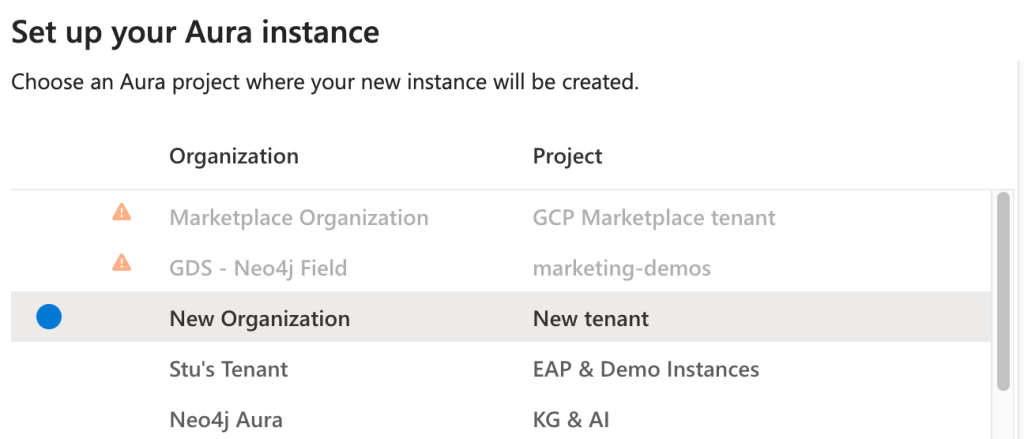
If you already have an AuraDB tenant you would like to use, you can use that or you can create a new tenant.

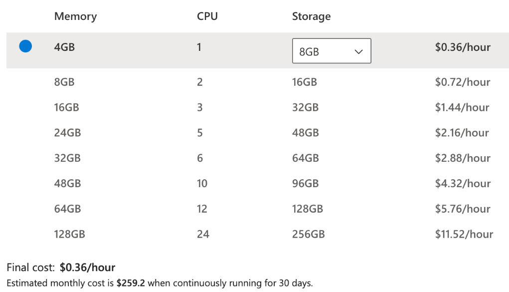
Then choose the memory you need. In our case, we can stick with the minimum.

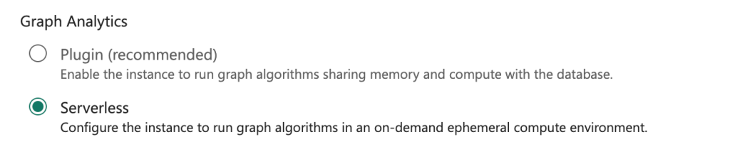
Because we’re mostly going to work in a notebook, we’ll choose Serverless, but if you’d prefer to use graph algorithms in AuraDB’s explore tab, choose Plugin.

Now that you’ve configured your instance, you should see a pop-up with your instance ID and password. Be sure to record those in a text file somewhere. We’ll need them later.

Create Your Graph Model

As promised earlier, we select the recommendations lakehouse. We’ll include all of our tables to transform into a graph.

The data import tool uses AI to automatically generate an initial graph model. In our case, it got it right on the first try, producing the following model.

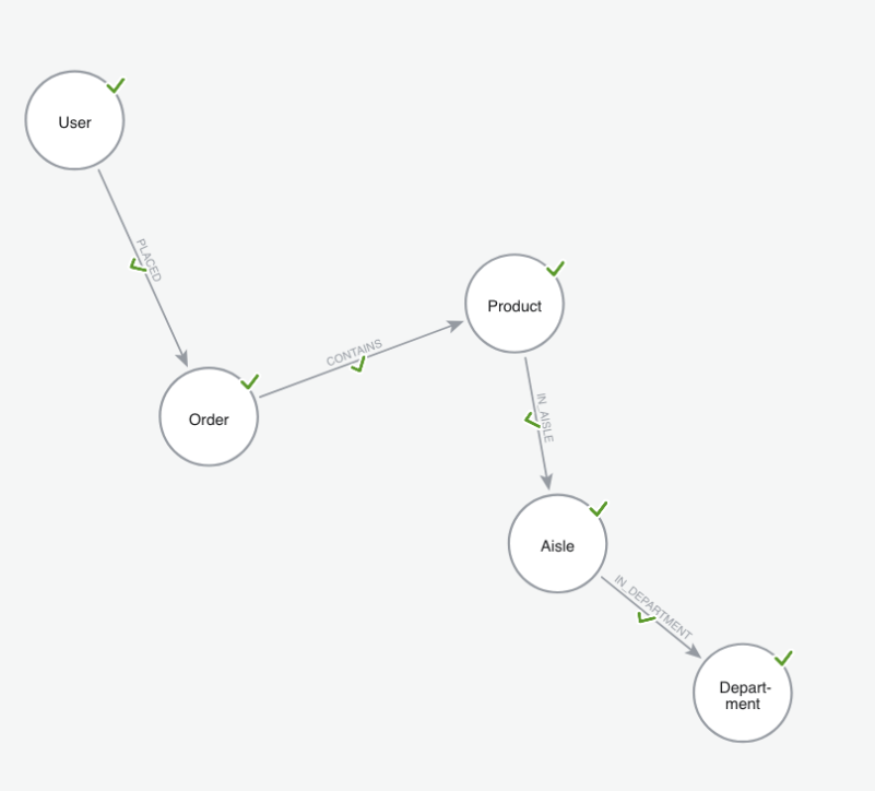
If you’re following along step by step, make sure you’re using the same graph model. Here’s what’s inside ours. Let’s start with the nodes.

Label	Property	Source Table	Source Column	Key
User	user	order_history	user_id	Yes
Order	Order	order_history	order_id	Yes
Product	productId	products	product_id	Yes
Product	name	products	product_name	No
Aisle	aisleId	aisles	aisle_id	Yes
Aisle	name	aisles	aisle	No
Department	departmentId	departments	department_id	Yes
Department	department	departments	department	No

And once you have your nodes, connect them with the following relationships.

Relationship	Source Table	From Node	From Id	To Node	To Id
PLACED	order_history	User	user_id	Order	order_id
CONTAINS	baskets	Order	order_id	Product	product_id
IN_AISLE	products	Product	product_id	Aisle	aisle_id
IN_DEPARTMENT	products	Aisle	aisle_id	Department	department_id

Note: Make sure all the property keys are integers.

Gathering Your Credentials

Next, we’ll need six pieces of information to connect Aura Graph Analytics to the database we set up.

For simplicity, we’ll store these values in a JSON file within the recommendations lakehouse. In a production environment, however, you should store your credentials securely in Azure Key Vault.

{
  "NEO4J_URI": "neo4j+s://<<YOUR_INSTANCE_ID>>.databases.neo4j.io",
  "NEO4J_USERNAME": "neo4j",
  "NEO4J_PASSWORD": "<<PASSWORD>>",
  "CLIENT_ID": "<<CLIENT_ID>>",
  "CLIENT_SECRET": "<<CLIENT_SECRET>>",
  "TENANT_ID": "<<TENET_ID>>",
}Code language: JSON / JSON with Comments (json)

Add the instance ID and password you generated when creating your instance in Fabric to the designated sections above.

Next, you’ll need your tenant ID. The easiest way to find it is by logging into Aura and checking the URL of the tenant that contains your Fabric instance. You can see which part of the URL to copy: https://console-preview.neo4j.io/projects/its-this-part-of-the-url/instances.

Finally, you need to create an API credential (follow the authentication instructions). 

Scoring Recommendations and Writing Back to OneLake

Next, we’ll create a Python notebook in Fabric. Before we start, we need to install the graphdatascience package.

Keep in mind: When you use pip install in Fabric, the package is only available for the duration of your current session. If your session times out or restarts, you’ll need to rerun the setup cells from the beginning.

%pip install graphdatascience

Next, we will load in all the packages needed to run our notebook:

from graphdatascience.session import DbmsConnectionInfo, AlgorithmCategory, CloudLocation, GdsSessions, AuraAPICredentials
from datetime import timedelta
import pandas as pd
import osCode language: JavaScript (javascript)

Now our secrets:

import json
with open("/lakehouse/default/Files/fabric_keys.json") as f:
    secrets = json.load(f)

NEO4J_URI = secrets["NEO4J_URI"]
NEO4J_USERNAME = secrets["NEO4J_USERNAME"]
NEO4J_PASSWORD = secrets["NEO4J_PASSWORD"]
CLIENT_ID = secrets["CLIENT_ID"]
CLIENT_SECRET = secrets["CLIENT_SECRET"]
TENANT_ID = secrets["TENANT_ID"]Code language: JavaScript (javascript)

Estimate resources based on graph size and create a session with a two‑hour TTL:

sessions = GdsSessions(api_credentials=AuraAPICredentials(CLIENT_ID, CLIENT_SECRET, TENANT_ID))

session_name = "demo-session"
memory = sessions.estimate(
    node_count=1000, relationship_count=5000,
    algorithm_categories=[AlgorithmCategory.CENTRALITY, AlgorithmCategory.NODE_EMBEDDING],
)

db_connection_info = DbmsConnectionInfo(NEO4J_URI, NEO4J_USERNAME, NEO4J_PASSWORD)Code language: JavaScript (javascript)

Then create a session:

gds = sessions.get_or_create(
    session_name,
    memory=memory,
    db_connection=db_connection_info, # this is checking for a bolt server currently
    ttl=timedelta(hours=2),
)

print("GDS session initialized.")Code language: PHP (php)

Items Commonly Purchased Together

For our purposes, we’re going to work with a subset of a co-purchase graph we create. We’ll see what items are purchased in the same market basket. But before we do that, let’s take a look at the top items that are purchased together:

query = """MATCH (o:Order)-[:CONTAINS]->(p1:Product),
      (o)-[:CONTAINS]->(p2:Product)
WHERE id(p1) < id(p2)
RETURN p1.product_name AS productA,
       p2.product_name AS productB,
       count(*) AS timesTogether
ORDER BY timesTogether DESC
LIMIT 5;"""

df = gds.run_cypher(query)
dfCode language: PHP (php)

productA	productB	timesTogether
Organic Baby Spinach	Banana	24
Bag of Organic Bananas	Organic Hass Avocado	22
Bag of Organic Bananas	Organic Strawberries	19
Banana	Organic Avocado	16
Organic Strawberries	Organic Hass Avocado	15

You’ll notice that four out of five of the top co-purchased pairs include bananas. Logically, I suppose this means that grocery stores should nearly always recommend bananas to customers – but should they really?

Let’s keep working through and see if that holds up.

Enter Node Similarity

When we recommend items, we should consider some items like hinges to others. If baby spinach and bananas are bought together and bananas and avocados are bought together, then perhaps someone who buys avocados also would want spinach.

But here’s the rub. If every grocery basket has bananas in it, then it isn’t a very good hinge. It doesn’t provide a personalized recommendation about what else someone might want to buy. When bananas are in every basket, their presence is not a good predictor of what other items will be in the basket. It’s just noise.

But before we can get a better recommendation, we need to create a projection. In our projection, we’ll create a co-purchase relationship between products weighted by the number of times products are purchased together:

if gds.graph.exists("copurchase")["exists"]:
    gds.graph.drop("copurchase")

query = """
CALL {
    MATCH (o:Order)-[:CONTAINS]->(p1:Product),
          (o)-[:CONTAINS]->(p2:Product)
    WHERE p1.product_id < p2.product_id
    WITH p1, p2, toFloat(COUNT(*)) AS weight
    RETURN p1 AS source, p2 AS target, weight
}
RETURN gds.graph.project.remote(
    source,
    target,
    {
        sourceNodeLabels: labels(source),
        targetNodeLabels: labels(target),
        relationshipType: 'CO_PURCHASED_WITH',
        relationshipProperties: {weight:weight}
        }

);
"""

copurchase_graph, result = gds.graph.project(
    graph_name="copurchase",
    query=query
)Code language: PHP (php)

We can then write these results back to our graph database:

result = gds.nodeSimilarity.write(
    copurchase_graph,
    topK=10,
    relationshipWeightProperty="weight",
    writeRelationshipType="SIMILAR_TO",
    writeProperty="score"
)Code language: JavaScript (javascript)

  If we take a look at our least similar pairs, we find that bananas often top the list:

query = """
MATCH (p1:Product)-[r:SIMILAR_TO]->(p2:Product)
RETURN p1.product_id AS product1_id, p1.name AS product1_name,
       p2.product_id AS product2_id, p2.name AS product2_name,
       r.score AS similarity_score
ORDER BY similarity_score 
LIMIT 10
"""

gds.run_cypher(query)Code language: PHP (php)

product1_id	product1_name	product2_id	product2_name	similarity_score
41162	Grapes Certified Organic California Black Seed…	13176	Bag of Organic Bananas	0.000856
41605	Chocolate Bar Milk Stevia Sweetened Salted Almond	13176	Bag of Organic Bananas	0.000856
31478	DairyFree Cheddar Style Wedges	13176	Bag of Organic Bananas	0.000856
46900	Organic Chicken Noodle Soup	24852	Banana	0.000887
45265	Raspberry on the Bottom NonFat Greek Yogurt	24852	Banana	0.000887

Persisting Results Back to OneLake

Here comes the easy part. We can easily write back to OneLake using Spark:

spark_df = spark.createDataFrame(df)
spark_df.write.format("delta").mode("overwrite").saveAsTable("scored_results")Code language: JavaScript (javascript)

What’s a Good Recommendation?

At this point, we’ve seen how to write back to OneLake and talked about what makes a bad recommendation – but what makes a good one? Let’s look at what coupons our system would suggest if a customer bought Peanut Butter Cereal (34), Organic Bananas (13176), and Cauliflower (5618).

Now that we have a OneLake table, other teams can query against that to find what items to recommend based on what is currently in the shopper’s basket. Here is what some SQL might look like to do so:

%%sql
WITH target_products AS (
    SELECT 34 AS target_id, 'Peanut Butter Cereal' AS target_name
    UNION ALL
    SELECT 13176, 'Organic Bananas'
    UNION ALL
    SELECT 5618, 'Cauliflower'
),
similarities AS (
    SELECT
        CASE 
            WHEN ps.product1_id = t.target_id THEN ps.product2_id
            ELSE ps.product1_id
        END AS similar_id,
        CASE 
            WHEN ps.product1_id = t.target_id THEN ps.product2_name
            ELSE ps.product1_name
        END AS similar_name,
        t.target_name,
        ps.similarity_score
    FROM scored_results ps
    JOIN target_products t
      ON ps.product1_id = t.target_id OR ps.product2_id = t.target_id
)
SELECT target_name, similar_name, similarity_score
FROM (
    SELECT
        target_name,
        similar_name,
        similarity_score,
        ROW_NUMBER() OVER (PARTITION BY target_name ORDER BY similarity_score DESC) AS rn
    FROM similarities
) ranked
WHERE rn <= 1
ORDER BY target_name, similarity_score DESC;Code language: PHP (php)

A weaker model might recommend something like Organic Strawberries, simply because they frequently appear alongside bananas. But a graph-based approach looks deeper. It recognizes that the similarity score for strawberries is driven by a universally popular item — bananas — which doesn’t tell us much about this specific shopper.

Instead, the algorithm surfaces Organic Pepper Jack Cheese, a connection rooted in cauliflower, an item that’s more distinctive to our customers’ preferences. In other words, node similarity filters out noisy, generic associations (like “bananas go with everything”) and highlights meaningful and personalized patterns.

Summary

With that, you’ve learned how to build a better recommendation, one that goes deeper than simply looking at which items are frequently purchased together. From this, you can recommend interesting and unique products your customers really want to buy.