Mastering Fraud Detection With Temporal Graph Modeling

Did you know that consumer credit fraud costs the financial industry more than $10 billion annually? With our customer (a top-tier French bank), we’re tackling this growing challenge head-on. Traditional methods struggle to keep pace with evolving fraud networks, prompting us to explore a dynamic and scalable solution: temporal graph modeling. In this post, we’ll dive into the problem, propose an innovative data model, and invite you to share your insights.

TL;DR

We built a scalable temporal graph model to compute point-in-time connected components in a User-Event-Thing graph in real time. The key insights:

1. Temporal CC Forest Model: Traditional weakly connected components (WCC) queries leak future information and can’t be used in real-time ML pipelines. We designed a dynamic graph structure where events are linked chronologically using :SAME_CC_AS relationships, forming a temporal forest of connected components. This preserves real-time graph state and avoids future leakage — perfect for ML training and fraud detection.
2. Optimized WCC batching: We first partitioned the graph with the Neo4j Graph Data Science WCC algorithm, then we use the connected component to route the whole connected subgraph to the same batch to process the forest data structure in parallel.
3. Replacing clique projections: Instead of projecting cliques, which explode in size around super-nodes, we projected linear paths to keep the graph sparse, avoiding O(n²) blowups.

The Problem: The Challenge of Dynamic Fraud

Consumer credit fraud manifests in forms like identity theft, coordinated account takeovers, and synthetic identities. Static rule-based systems often miss these patterns because fraud networks evolve over time — shared IPs or credit cards might link dozens of accounts gradually. For instance, a fraud ring could emerge over a year, requiring us to capture the state of these connections at the moment an event is flagged.

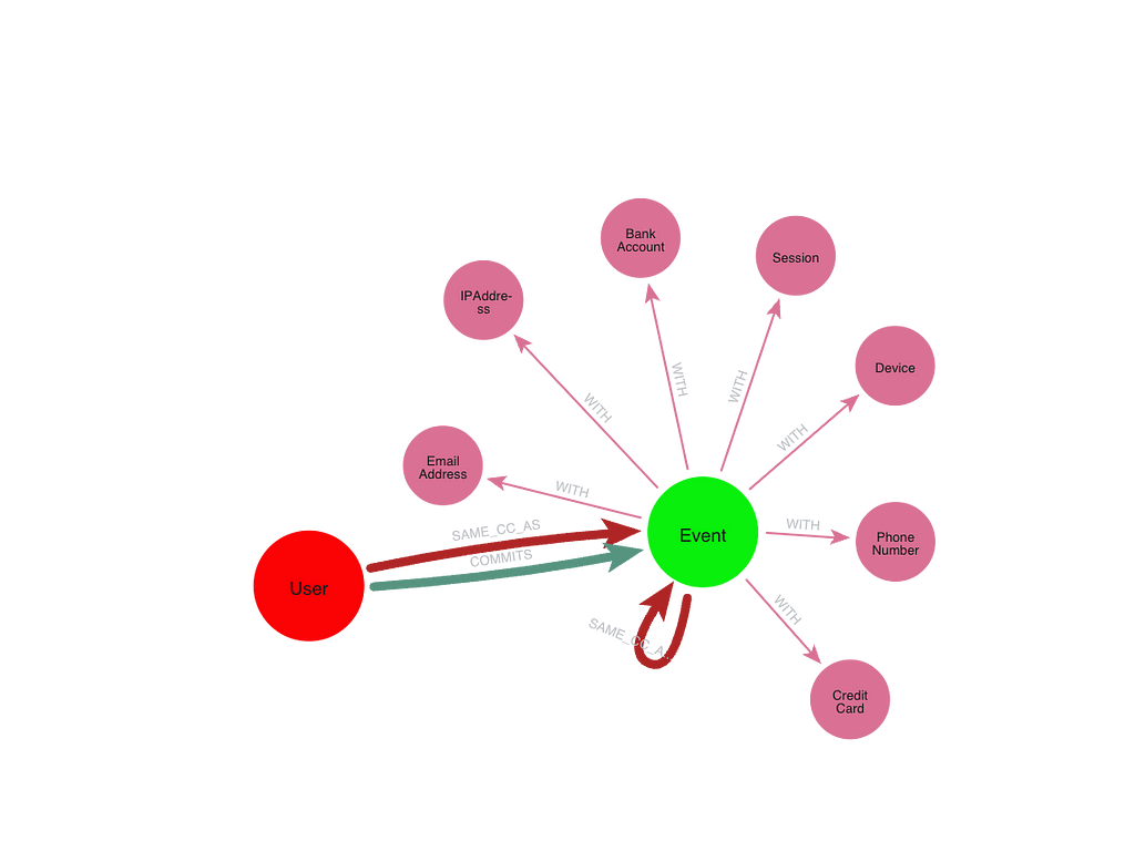
Imagine a fraud graph with three main node types:

(:User)-[:COMMITS]->(:Event)-[:WITH]->(:Thing)

• User: The actor
• Event: An application, transaction, or login
• Thing: Shared resources — phone numbers, IPs, devices, emails, etc.

Fraud rings are made of users that share Things in a way that connects them. The idea is to compute connected components (CCs) and extract features from them — size, density, fraud ratio — as input to a machine learning model.

Why Time Matters

Time is critical. A static snapshot of the graph fails to reflect how relationships build progressively. Imagine a fraud cluster forming over months, with new users joining via shared entities. Without a temporal view, we risk missing these dynamics, making real-time detection nearly impossible.

Real-time fraud detection machine learning model training requires that features are computed as of the moment an event occurs. So components must be temporal: An event should only belong to a component that existed up to its timestamp — no foresight allowed.

We initially tried using a time-slice approach, leveraging Graph Data Science WCC to compute connected components. But this introduced a critical flaw: future leakage. Because WCC doesn’t account for time, events could end up in the same component even if they were only indirectly connected by future actions. In effect, an event could be classified using information that didn’t exist at the time — violating real-time constraints.

This was a deal-breaker for our machine learning pipeline. We needed to compute feature vectors that represented the graph state exactly as it appeared when each event occurred. If components included future knowledge, model training would be biased, and validation would produce misleadingly high scores. That’s not just bad science — it’s unusable in production.

So, we needed a model where each event is assigned to a connected component that reflects only the information available at the time it happened. No foresight. No leakage. Just clean, temporal structure.

Our Approach: A Time-Forest Data Model

To address this, we propose a time-forest data model. This structure represents connected components as a forest where:

• Leaves are User nodes.
• Inner nodes are Event nodes that may add new connections.
• Roots are Event nodes identifying the current connected component.

This allows us to query the state of a component as of a specific date efficiently, capturing all relevant users and events at that moment. Unlike simple temporal indexing, it preserves the evolving network structure.

Implementation in Neo4j

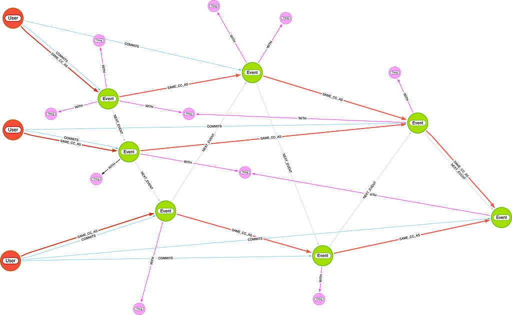
Let me introduce a CC forest data model using :SAME_CC_AS relationships between User and Event nodes, always pointing forward in time.

Each User starts as its own ConnectedComponent. As events are processed (chronologically), each one gets connected to:

• The last ConnectedComponent node :SAME_CC_AS — reachable from the User who commits the Event
• The last ConnectedComponent node :SAME_CC_AS — reachable from an Event node sharing a Thing with the current Event

The processed Event is given the ConnectedComponent as a second label.

Understanding :SAME_CC_AS — Temporal Component Linking

The :SAME_CC_AS relationship is the backbone of the temporal connected component forest. It links events chronologically to build a time-respecting view of user interactions and shared resources.

For each new Event node, we determine which past component(s) it should belong to based on who triggered it and what Things it’s linked to. We then connect it to the most recent terminal event of those components using the new :SAME_CC_AS relationship.

Following are two examples.

Example 1: Simple Login Event

If user u logs in, triggering an event e, we locate the most recent connected component that u belongs to by following (u)-[:SAME_CC_AS]->*(last), then connect that last event to e: (last)-[:SAME_CC_AS]->(e).

This links e to the same evolving component as u, ensuring continuity.

Example 2: Update Involving Shared Resource

Now suppose u updates their email address, and that change is recorded in a new event e. The email (Thing) is already connected to past events e₁, e₂, …, eₖ.

We now consider multiple origins for connected components:

• From the user: (u)-[:SAME_CC_AS]->*(last_from_u)
• From each related event eᵢ: (eᵢ)-[:SAME_CC_AS]->*(last_from_ei)

We then connect all these terminal events to e:

• (last_from_u)-[:SAME_CC_AS]->(e)
• (last_from_e1)-[:SAME_CC_AS]->(e)
  …
  (last_from_ek)-[:SAME_CC_AS]->(e)

This ensures that e merges multiple previously separated components into a single one, while preserving temporal causality.

Building the Structure: First Query

Here’s a query to build such a structure in our model:

CYPHER 5
MATCH (e:Event&!ConnectedComponent)
WITH e ORDER BY e.timestamp
CALL (e) {
  MATCH (e)(()-[:WITH]->(entity)<-[:WITH]-(:ConnectedComponent)
){0,1}()<-[:COMMITS]-(u)
  WITH DISTINCT e, u
  MATCH (u)-[:SAME_CC_AS]->*(cc WHERE NOT EXISTS {(cc)-[:SAME_CC_AS]->()})
  MERGE (cc)-[:SAME_CC_AS]->(e)
  SET e:ConnectedComponent
} IN TRANSACTIONS OF 100 ROWS

Results and Insights

The time forest enables localized, as-of-date queries, revealing fraud patterns. Let’s see some examples:

// Get all connected components as-of a given date
CYPHER 5 runtime=parallel
MATCH (cc:Event)
  WHERE cc.timestamp <= $asOfDate
  AND NOT EXISTS {
    (cc)-[:SAME_CC_AS]->(x:Event WHERE x.timestamp <= $asOfDate)
  }
RETURN cc

// Get a connected component from an event_id, with context
MATCH p=(u:User)(()-[:SAME_CC_AS]->(ev))*(e:Event {event_id:$event_id})
UNWIND ev+[e] AS event
RETURN p, [(event)-[r:WITH]->(x)| [r, x]] AS with_things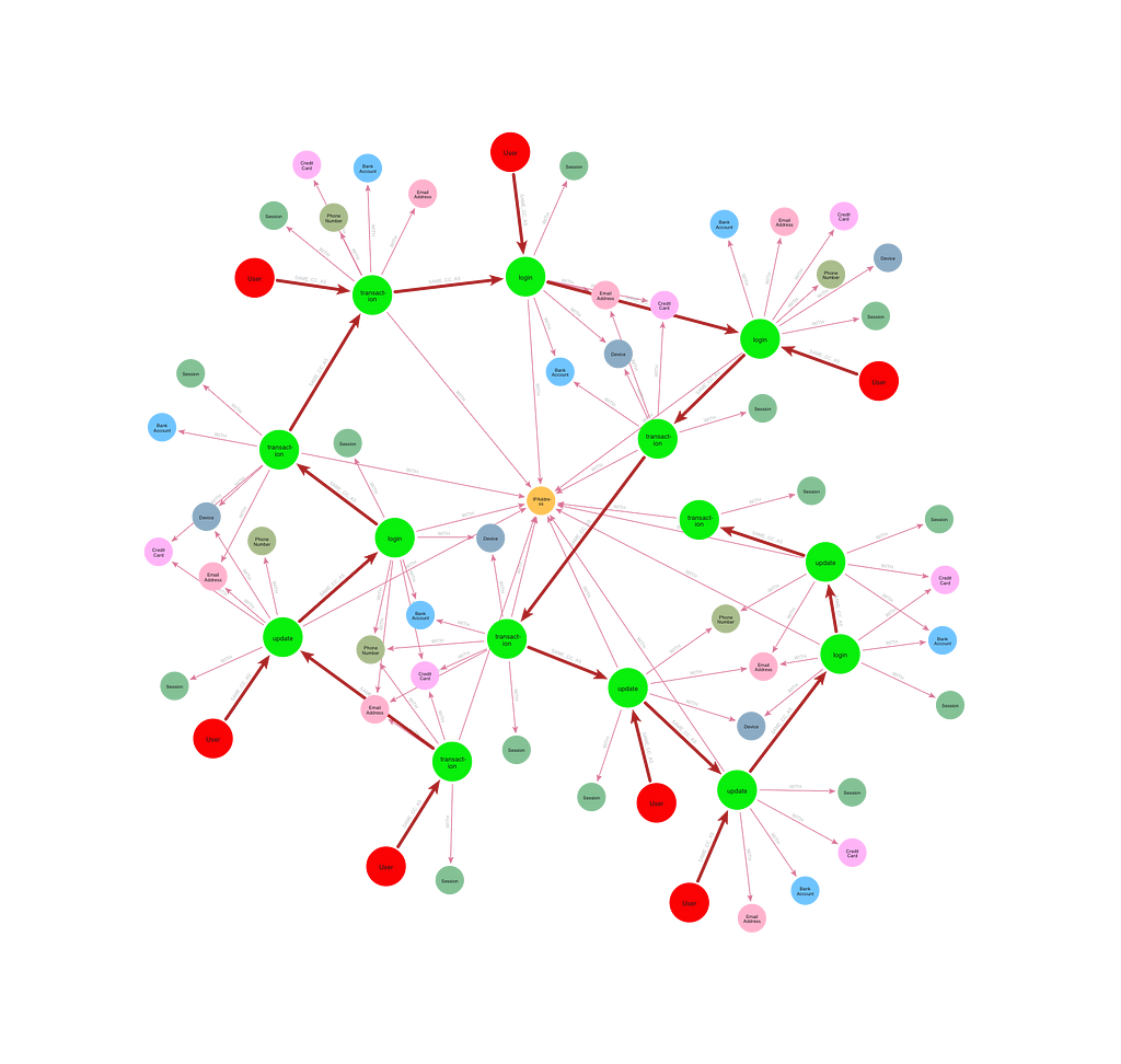

// generate consistent sample dataset with no future leakage
CYPHER 5
MATCH (e:Event)
WITH e, rand() AS random_rk
ORDER BY random_rk
LIMIT $sample_target_size
MATCH (u:User)-[:SAME_CC_AS]->*(e:Event)
RETURN collect(u) AS users_in_cc, e
ORDER BY size(users_in_cc) DESC

// generate user-based sampling as of date
CYPHER 5
MATCH (u:User)
WITH u, rand() AS random_rk
ORDER BY random_rk
LIMIT $sample_target_size
MATCH (u)-[:SAME_CC_AS]->*(cc:Event
  WHERE cc.timestamp <= $asOfDate
  AND NOT EXISTS {(cc)-[:SAME_CC_AS]->(x:Event WHERE x.timestamp <= $asOfDate)}
  )
WITH DISTINCT cc
CALL (cc){
  MATCH (u:User)-[:SAME_CC_AS]->*(cc)
  RETURN u
} IN CONCURRENT TRANSACTIONS OF 10 ROWS
RETURN u, cc

You can sample connected components at a point in time, extract features, and label them. But it only works if events are processed sequentially, which can lead to an inefficient one-threaded building of the data structure. We still need to optimize the process.

First Optimization: Parallel Processing With Graph Data Science WCC

Chronological processing doesn’t scale. As events and component sizes grow, building the structure becomes increasingly slow. Because each event depends on the state of the graph up to its timestamp, events must be processed in strict chronological order to ensure correctness. This makes it inherently sequential — a single event could change the component structure in a way that affects all following events. Without partitioning, you can’t safely parallelize without risking incorrect component assignments.

However, when I demonstrated the model to my colleague Maxime Guery, he had a killer insight:

“If you precompute the final weakly connected components with Graph Data Science, you can process each one in isolation. Parallelism for free.”

He was right. Using the Graph Data Science WCC algorithm:

CYPHER 5
CALL gds.wcc.stream('wcc_graph')
YIELD nodeId, componentId
WITH gds.util.asNode(nodeId) AS event, componentId
WITH componentId, collect(event) AS events
ORDER BY rand() // shuffle components to balance batch size
CALL (events) {
  UNWIND events AS e
  WITH e
  WHERE NOT e:ConnectedComponent
  ORDER BY e.timestamp ASC
  CALL (e) {
    MATCH (e)(()-[:WITH]->(entity)<-[:WITH]-(:ConnectedComponent)
  ){0,1}()<-[:COMMITS]-(p)
    WITH DISTINCT e, p
    MATCH (p)-[:SAME_CC_AS]->*(cc WHERE NOT EXISTS {(cc)-[:SAME_CC_AS]->()})
    MERGE (cc)-[:SAME_CC_AS]->(e)
    SET e:ConnectedComponent
  }
} IN CONCURRENT TRANSACTIONS OF 100 ROWS

WCCs partition the graph into disjoint subgraphs. Since no event connects across WCCs, they don’t connect across batches. You can safely build temporal components inside each in parallel.

Second Optimization: Killing the Clique Explosion

There was one big issue left. The Graph Data Science WCC projection step was expensive — RAM-hungry and slow. Why?

The in the naive way to do this, projecting the source-->target relationship for each (source)-[:WITH]->(t:Thing)<-[:WITH]-(target)match, each Thing (e.g., a phone or IP) becomes a clique in the projected graph: countingO(degree(t)^2) relationships. With popular shared entities, this becomes unmanageable.

The twist: I don’t need full cliques.

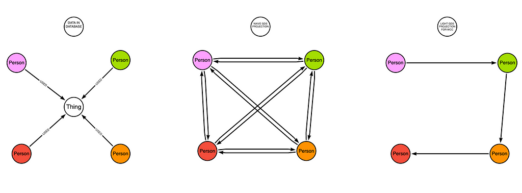
To compute WCCs, we just need reachability. So I projected a path instead of a clique:

CYPHER 5
MATCH (thing:Thing|User)
CALL (thing) {
  MATCH (e:Event)-[:WITH|COMMITS]-(thing)
  WITH DISTINCT e
  WITH collect(e) AS events
  WITH CASE size(events)
    WHEN 1 THEN [events[0], null]
    ELSE events END AS events
  UNWIND range(0, size(events)-2) AS ix
  RETURN events[ix] AS source, events[ix+1] AS target
}
RETURN gds.graph.project(
  'wcc_graph', source, target, {});

This preserves connectivity (same WCCs), but drastically reduces edge count from O(degree(t)^2) to O(degree(t)) per Thing. Now even huge graphs project in seconds.

Final Words

Temporal connected components turned out to be a powerful structure for graph-based fraud detection — especially when used as a feature generator for machine learning.

Maxime Guery’s idea to use Graph Data Science WCCs for safe parallelism, and our sparse-path projection trick to kill clique growth, made this model fast, scalable, and production-ready. Those tricks turned previously impossible queries into feasible ones for real-time workloads, and transformed multi-hour, high-resource batch jobs into operations that complete in seconds — even in modest environments.

Want to try it yourself? You can download a dataset and play with these queries. Everything is available on GitHub.

Temporal graph modeling, enhanced by our time-forest approach, tackles the dynamic nature of credit fraud. Have you faced similar challenges? Share your thoughts or join us in refining this model!

Be sure to learn more about Neo4j Graph Data Science.

---

Mastering Fraud Detection With Temporal Graph Modeling was originally published in Neo4j Developer Blog on Medium, where people are continuing the conversation by highlighting and responding to this story.