Exploring Neo4j Spatial: Installation, Data Loading, and Simple Querying

Product Manager, Neo4j

July 23, 2025

10 min read

Introduction

The common division of responsibility between graph databases and GIS platforms limits the ability to exploit the full power of graph databases and graph query languages like Cypher to effectively explore relationships that involve both geospatial and non-geospatial relationships.

This series of blogs will cover:

Installation, data loading, and simple querying
Layer management, spatial filtering, and intersection
Path intersections using AIS data
Custom procedures for spatial analysis

In this first blog, I’ll look at Neo4j Spatial and explore how effective it can be in integrating spatial analytics into Cypher graph queries.

Background

Conceptually, graph databases and geospatial analysis are a natural fit, as both focus on the relationships and connectivity between data points. In geospatial analysis, we’re often interested not just in where things are but how they relate to each other — adjacency, containment, proximity, movement through space, networks (like roads, rivers, pipelines, or flight paths).

Neo4j is built to efficiently model and query these kinds of connections. Every node (representing a place, object, or event) and every relationship (like crosses, adjacent to, within, near) can be stored explicitly and queried flexibly. This means you can easily ask complex questions with much less overhead than traditional relational or GIS databases, which typically aren’t optimized for deep relationship traversal.

Despite this strong conceptual alignment, geospatial analysis is often conducted outside of Neo4j using dedicated GIS tools — with the graph database reserved for primarily non-spatial operations. This separation is unfortunate. Moving data back and forth between systems can introduce inefficiencies, delays, and opportunities for inconsistency. More importantly, keeping spatial and non-spatial analysis apart means missing out on the full power of graph queries — where spatial relationships (like proximity or containment) can be combined directly with non-spatial patterns (such as financial transactions, communication links, or organizational hierarchies) to uncover deeper insights.

By bringing geospatial and non-geospatial data together in the same graph, analysts can ask much richer questions. For example, we might think about the sort of complex questions an analyst working in maritime security and fraud detection might need to ask — perhaps looking at illicit behaviors like illegal oil transfers, smuggling, sanction evasion, or money laundering.

Graph databases are widely used to uncover hidden patterns, such as non-obvious financial relationships, vessel ownership hidden via offshore companies, or payments routed through multiple banks. However, maritime security analysts might typically also want to ask questions of the data that are explicitly geospatial. For example, to detect:

Anomalous movement patterns (such as circling, loitering, unusual speed changes)
Identify spoofing (anomalous position, duplicate transmissions)
Zone intrusion (vessels straying into marine protected areas, no-fishing zones)
Unusual shipping routes (non-standard routes between ports, avoidance of main shipping lanes)
Dark activity (AIS transponder gaps)
Illegal refueling (detected by long proximity events between vessels)

Neo4j and Geospatial

Neo4j’s core geospatial capabilities are built into the database natively, without needing a separate plugin. These capabilities mainly focus on working with points (latitude/longitude, as well as Cartesian coordinates), distance calculations, and basic spatial predicates inside Cypher. Neo4j doesn’t natively support other geometry types (lines and polygons for example), or non-geographic coordinate reference systems. To work with these data types, and to perform more sophisticated geospatial graph analysis, we must turn to Neo4j Spatial.

Neo4j Spatial originated in 2010 as an open-source extension to add geospatial capabilities to Neo4j. Developed primarily by Craig Taverner and contributors, it allowed users to model and query spatial data (points, lines, polygons) directly inside Neo4j using spatial indexes, inspired by GIS systems. The plugin has recently been ported to work with Neo4j 5.x, and a 2025.x release is pending.

Neo4j Spatial Steps

In this first part of the series, I begin with the basics — simply loading some polygon data into Neo4j. The sample data for all the examples is on GitHub. This is a multi-part ZIP archive, so you’ll need a tool to extract the contents.

Installation

To start, we need to install the plugin. You can download the latest version on GitHub. You’ll need the one named neo4j-spatial-x.xx.x-server-plugin.jar. Make sure to download the file appropriate to the version of Neo4j you’re running. The plugin is periodically updated, and the most recent version at the time of writing is neo4j-spatial-5.26.0-server-plugin.jar, which targets the Neo4j server release 5.26 (Long-Term Support version).

Copy the plugin into your database plugins folder, then update the neo4j.conf file to whitelist the spatial procedures. You do this by appending spatial.* to the config setting dbms.security.procedures.unrestricted and (only if it is set) to dbms.security.procedures.allowlist. Then restart Neo4j for these changes to take effect. Test that the plugin has loaded correctly:

SHOW PROCEDURES where name STARTS WITH "spatial."

Layers

The spatial plugin borrows the idea of geospatial layers from GIS applications. A layer can hold data of only one spatial type, such as point, linestring, polygon, or multipolygon.

So we begin by creating a layer into which I’ll load a file containing the boundary polygons of U.K. administrative areas:

CALL spatial.addLayer('admin_areas', 'wkt',"","")

The spatial plugin needs us to specify which encoder to use for the layer we’re creating. Our options include well-known text (WKT) and well-known binary (WKB). These are Open Geospatial Consortium (OGC) standard formats intended for passing simple geometry information between applications. We’ll use WKT, as this format stores feature geometry as a string in a geometry property. WKT is human-readable, so it’s easy to work with when debugging. Please note that WKT property strings can become extremely long when encoding large geometries.

We can check that our layer has been added with CALL spatial.Layers, which returns a list of spatial layers registered in the database. Having successfully created a layer, we can take a look at what that actually looks like in the database.

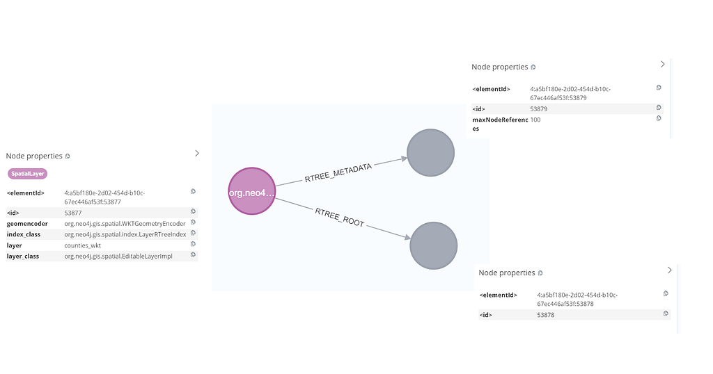
The spatial.addLayer procedure creates a SpatialLayer node, which is connected via an :RTREE_ROOT relationship to the root node of the spatial index that has also been created for us, and which will manage the data we load. There is also an :RTREE_METADATA relationship, linking to a node that manages essential metadata for the maintenance of the spatial index, including the maximum number of references that can be connected to a root node. As we add data to our layer, additional child nodes will be created, as we will see below.

Import Data Into a Layer

Our layer is currently empty, so we need to add some data. The spatial plugin import procedures support a few file-based spatial data formats: Shapefile, OpenStreetMap, WKT, WKB and GeoJSON:

spatial.importShapefile (with encoders for WKT, WKB, and GeoJSON)
spatial.importShapefileToLayer
spatial.importOSM
spatial.importOSMToLayer
spatial.addWKT
spatial.addWKTs

I’m going to add a shapefile containing U.K. administrative area boundaries — part of the free data provided by the Ordnance Survey. I’d previously converted this into WGS 84 geographic coordinates, and that’s what I’ll use here. The preprocessed data can be downloaded using the link above, though the original (free, open) source data can be downloaded from Ordnance Survey.

To simplify this demonstration, where some of the features in the dataset are multipart polygons, I’ve pre-processed these into single-part polygons, and also converted them into the WGS 84 geographic coordinate system. For the examples below, please use that version, which you can download:

CALL spatial.importShapefileToLayer("admin_areas", "import\OS_admin_areas_WGS84")

This completed in 8 seconds on my laptop, telling me that 350 records were loaded. I’m running on an i9 processor, so that seems a bit slow, though shapefiles are a complex format, requiring the plugin to read and join geometry and attributes held in multiple files, so there’s quite a lot of heavy lifting going on behind the scenes.

Let’s look at what that did to our spatial layer and the spatial index:

CALL spatial.layer("admin_areas") YIELD node AS layerNode
RETURN layerNode

Expanding our layerNode in the browser UI shows that the root index node now has five child nodes, each with a bounding box (bbox) property.

The bounding box coordinates record the combined extent of all of the spatial features stored in that branch of the (R-tree) index. When new records are added to the index, Neo4j Spatial will add the record to the index leaf that contains the bounding box that would expand the least — so it tries to cluster similar geometries together adaptively. It’s this R-tree structure that enables the plugin to return spatial queries (nearest, contains, intersects) rapidly.

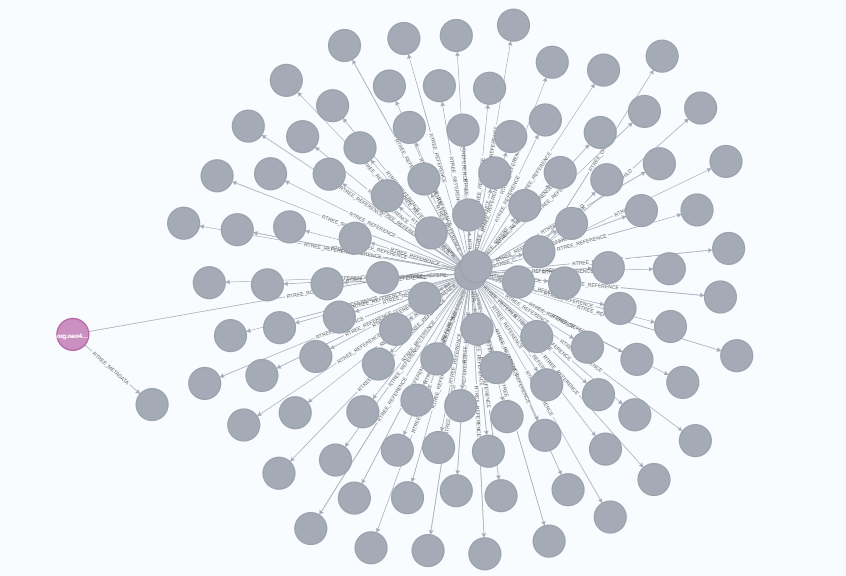
Expanding one of the child index nodes shows us that it’s connected by a RTREE_REFERENCE relationship to dozens of reference nodes, each containing the metadata of a single feature from our imported admin area dataset.

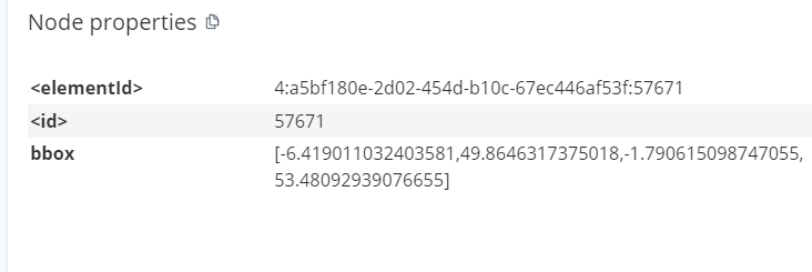
Following is an example of the properties stored on a single reference node.

From this, we can see that the plugin has successfully imported the properties from the shapefile’s .dbf file and stored these as properties on individual spatial feature nodes.

I thought it would be a good idea to check that the geometry was loaded properly by trying a simple intersection query. To do this, I’ll pass a polygon that covers a large area of southern Britain into the query. The query should find several features in my admin area layer that intersect my simple polygon, then convert the output (using spatial.asGeometry) into a geometry representation that I can read:

WITH 'POLYGON((-2 50, -1 50, -1 51, -2 50))' AS polygon // area in southern Britain
CALL spatial.intersects('admin_areas', polygon) YIELD node // data features that intersect my defined area
CALL spatial.asGeometry(node.geometry) YIELD geometry // get geometry of intersecting areas
RETURN geometry

However, this returned an error:

Failed to invoke procedure `spatial.asGeometry`: Caused by: java.lang.RuntimeException: Can't convert MULTIPOLYGON (((-1.3103777877257892 50.76736153454187, -1.3102438964376912 50.76735399877745, -1.3101288626393064 50.76736590913311, -1.3100222370090933

This is telling me that although the intersection calculation was successful, the spatial.asGeometry procedure cannot handle MULTIPOLYGON structures. (Read more about the difference between simple polygons and multipolygons.)

At this stage, it’s worth saying a bit more about the WKT format. WKT can be used to store a range of different geometry types (gtypes), each of which has an associated code, which the plugin stores as a property alongside the geometry.

You can see in the properties for the Somerset feature example above that the gtype is indeed 6 (multipolygon), whereas the spatial.asGeometry procedure requires a simple polygon (gtype 3). I’ll need to go back to my GIS project and re-export my admin_areas layer as polygons rather than multipolygons.

Unfortunately, it seems that my GIS software of choice, QGIS, doesn’t give me control over this and always exports shapefile polygons as multipolygons. My workaround will be to export the admin_areas data as CSV, storing the simple polygon geometry as text in WKT format. I’ll then import this into Neo4j using LOAD CSV, rather than using the shapefile encoder.

The CSV file I created and used for the examples (again based on the free and open Ordnance Survey Boundary-Line source data) can be downloaded, though again, you can download my pre-prepared dataset.

So, I’ll delete the existing admin_areas layer, which also removes all the data I previously imported into that layer:

CALL spatial.removeLayer("admin_areas")

And start again:

CALL spatial.addLayer(admin_areas, 'wkt',"","")

Loading all this data with LOAD CSV is likely to take significant time. Luckily, we can use parallel load capabilities provided by CALL {} IN CONCURRENT TRANSACTIONS and make use of all the cores in my laptop:

:auto // this is required if you run CALL IN TRANSACTIONS queries using Browser
LOAD CSV WITH HEADERS FROM 'file:///admin_areas.csv' AS row
WITH row.WKT AS wkt, row.name AS name, toInteger(row.id) AS id
WHERE wkt IS NOT NULL AND wkt <> '' // ✅ Skip empty WKT values
CALL {
WITH wkt, name, id
CALL spatial.addWKTs('admin_areas', [wkt]) YIELD node
SET node.name = name, node.id = id
} IN CONCURRENT TRANSACTIONS OF 1000 ROWS;

I have 16 processor cores on my laptop, and this change gives me an almost 16x performance improvement over the same query run without CALL {} IN CONCURRENT TRANSACTIONS — with the import completing in 25 seconds. This is still slower than the 8 seconds it took to load the data using the shapefile loader, but that’s acceptable until I find a way to export my shapefiles as single-part rather than multipart — but that challenge will have to wait for another day.

Note: If you encounter memory issues when running this example on a machine with less RAM than I had available, you can open neo4j.conf and change the db.import.csv.buffer_size setting to a larger value.

Summary

So far, we’ve discussed why geospatial data and graph databases are a perfect match and how to get advanced geospatial functionality in Neo4j by installing Neo4j Spatial. We have looked briefly at the plugin’s index structure and learned how to create a layer and populate it with data. We’re now ready to start working with the data we loaded. That’ll be the subject of the next part of this blog. Stay tuned!