Solve Scheduling Problems With Relationship Coloring and Neo4j

Introduction

Some things really must be done one at a time, even though many of us like to think we can multitask. When multiple entities interact but can only interact with one other entity at a time, we can model the problem as a graph. Nodes in the graph represent entities, and relationships represent their interactions. Relationships can be colored to represent different time windows. The requirement that entities cannot have multiple interactions at the same time maps to a graph requirement that no node can be connected to multiple relationships of the same color.

Planning the Big Ten Football Schedule

Planning the Big Ten Conference regular season college football schedule is an example of a scheduling problem that can be represented as a relationship coloring problem. There were 18 teams in the conference in 2024, and each team played nine games against other teams in the conference. Each team played at most one game per week.

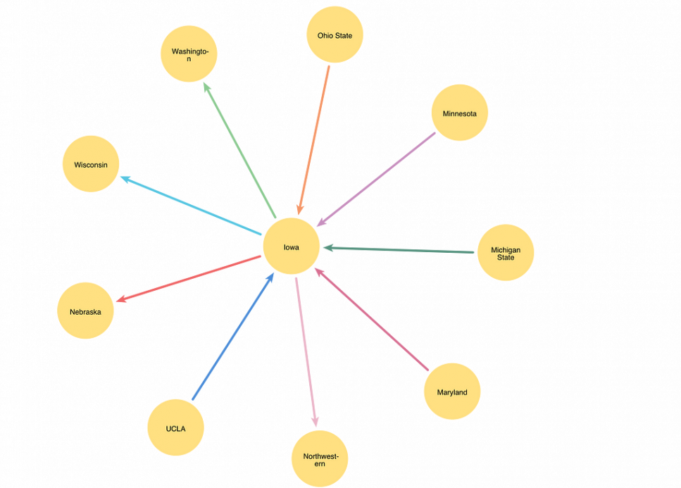
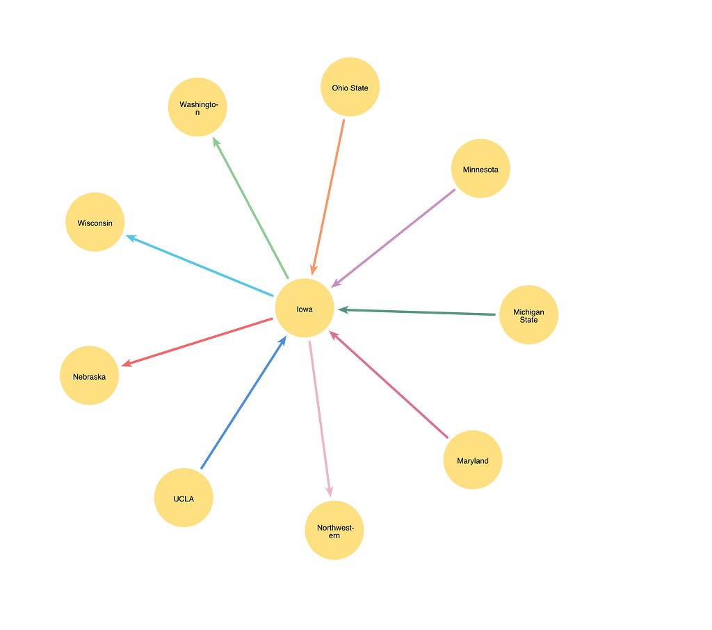
I loaded a graph of the 2024 Big Ten season into Neo4j. Each Team node represents a team in the conference, and each PLAYS relationship represents a game that needs to be scheduled. Each PLAYS relationship will be assigned a color property indicating the color assigned to the relationship. The subgraph below shows games played by the University of Iowa. The different colored relationships indicate that the games all take place during different weeks of the season.

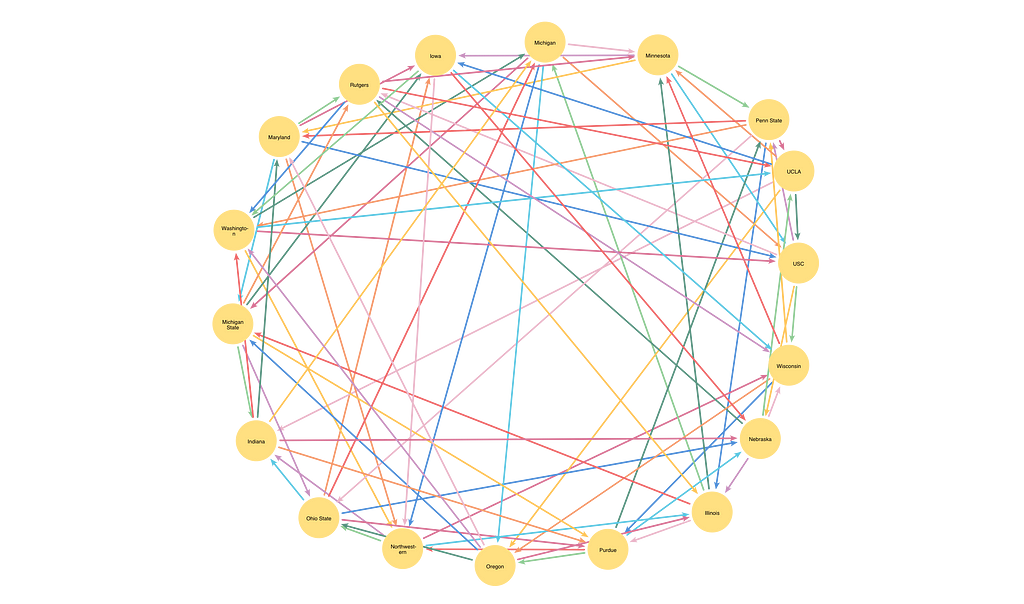
Here is a possible coloring for the whole graph representing all 18 teams in the conference based on the opponents they played in the 2024 season.

Steps

Implementing the Misra and Gries Relationship Coloring Algorithm

Misra and Gries described an algorithm for coloring simple graphs that completes in polynomial time. Their algorithm is based on Vizing’s theorem. Beginning from a graph where no relationships are colored, the algorithm colors one relationship at a time until all relationships are colored. Each iteration of the algorithm leaves the graph in a state where no node adjoins two relationships of the same color.

I implemented the Misra and Gries algorithm in Python and Neo4j. The code is available on GitHub. Neo4j makes it easy to keep track of the state of the graph and to visualize the results of the relationship coloring. Quantified path patterns, a feature of Neo4j’s Cypher graph query language, are useful in finding chains of relationships with alternating colors in one step of the algorithm.

Finding the Number of Colors for Your Graph

When coloring the relationships in a graph, we might begin by wondering how many colors we will need. A node’s degree means the number of relationships that have that node as an endpoint. Since all relationships connected to a single node must have different colors, we know it’ll require at least as many colors as the degree of the highest-degree node in the graph to color the graph. How many more than the maximum degree are needed? Vizing’s theorem guarantees that for a simple graph, where a pair of nodes can be connected by at most one relationship, the maximum number of colors required to color the relationships is the highest degree of any node in the graph plus one.

Since all nodes in the Big Ten graph have nine neighbors, we know that we can color the Big Ten football graph with at most 10 colors. Teams generally take at least one week off during the football season, so 10 colors seems like a realistic coloring for this graph.

This Python code queries Neo4j to get a list of integers representing the colors for the graph:

def get_colors():
    records, _, _ = driver.execute_query("""
        MATCH (n:Team)-[:PLAYS]-()
        WITH n, count(*) AS degree
        WITH max(degree) AS maxDegree
        RETURN range(1, maxDegree+1) AS colors
                         """)
    return records[0]['colors']

Gathering Relationships for Coloring

Next, we gather a list of all relationships in the graph. We don’t care about relationship direction when coloring the graph, but we need distinct names for the two endpoints of the relationship we are coloring. In this query, we give one endpoint the variable name x and the other endpoint the variable name f1. This query returns all the uncolored relationships so you can use it if you’re starting from a partially colored graph.

records, _, _ = driver.execute_query(
  """MATCH (x)-[r:PLAYS]->(f1) 
  WHERE r.color IS NULL 
  RETURN x.name AS x, f1.name AS f1""")
rels = [(record['x'], record['f1']) for record in records]

We will say that a color is free on a node if there’s not already a relationship of that color adjacent to that node. In our football graph, a color represents a weekend of the season, and a color is free for a team if that team doesn’t already have a game scheduled for that weekend.

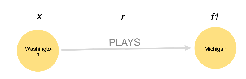
No relationships are colored in the first iteration of the algorithm. All weekends are available for all teams. Any choice of a color for the first relationship will leave the graph in a valid state. As the iterations progress, coloring becomes more complex because there are more colored relationships that might conflict with any new relationship coloring. We’ll walk through an iteration of the Misra and Gries algorithm on a partially colored graph. This iteration will find a color for the game between Washington and Michigan. We’ll call the relationship that we want to color r.

Finding a Maximal Vizing Fan

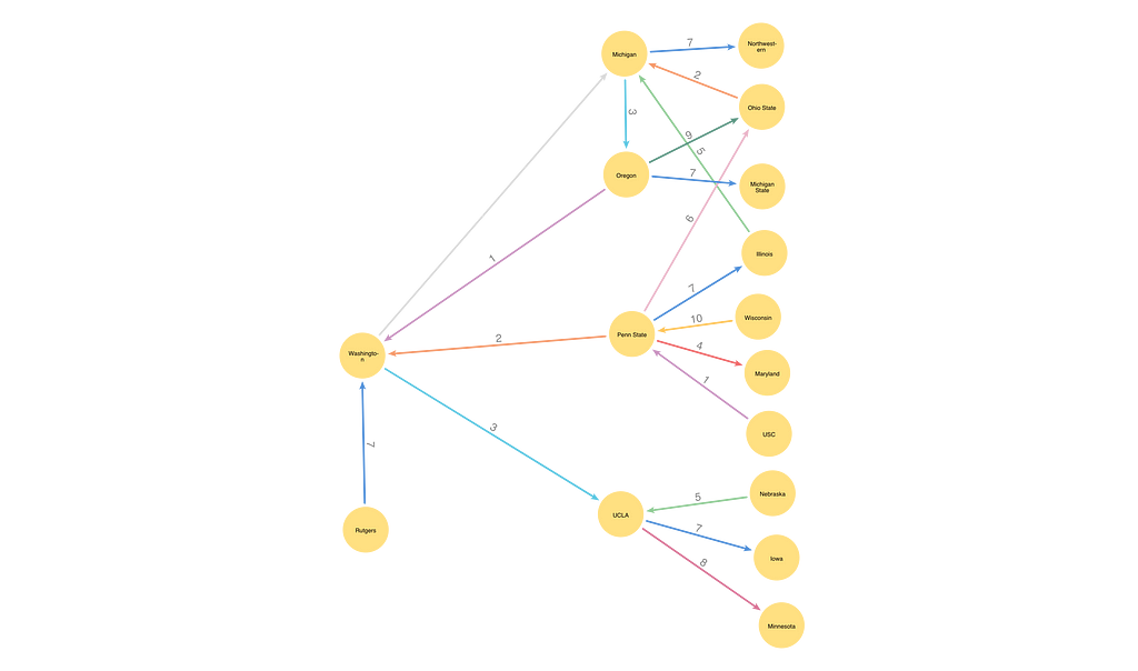
We’ve called one of the nodes adjacent to our relationship x. In our example, x is Washington. We begin the coloring process by finding a Vizing fan for x. A Vizing fan is a list of neighbors of x, beginning with the other node related to r, which we labeled f1. For each node added to the fan, the color of the relationship between x and the previous member of the fan must be free on the new member. We continue adding nodes to the fan until no more neighbors of x meet the criteria for addition to the fan.

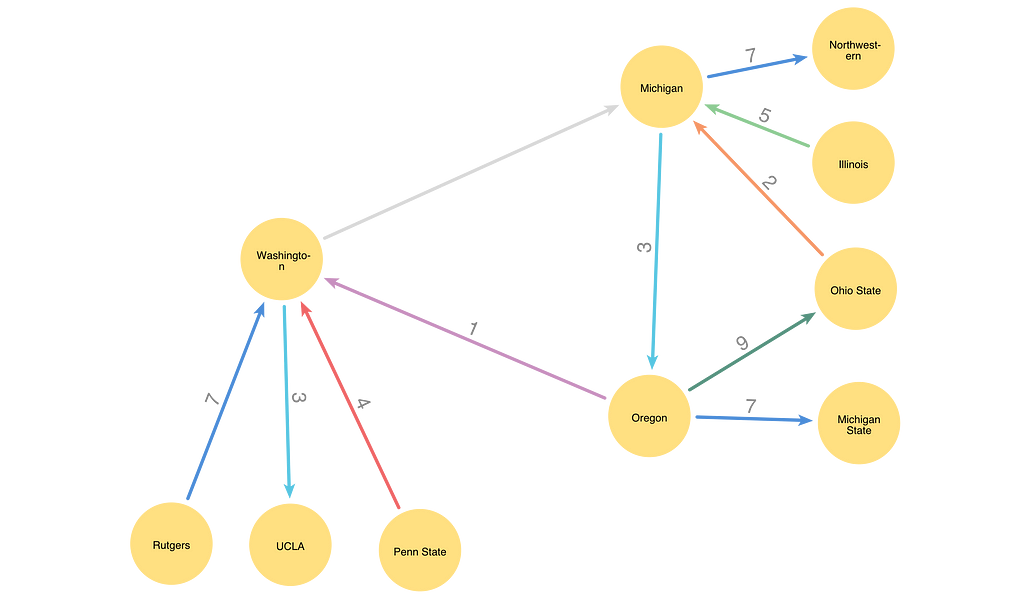
Below, we want to color the Washington-Michigan relationship, so the fan begins with Michigan. We can add Oregon as the second fan member. The color of the Washington-Oregon relationship (1) does not conflict with the existing Michigan-adjacent colors (2, 3, 5, 7). We can add Penn State to the fan after Oregon because the color of the Washington-Penn State relationship (2) does not conflict with the colored relationships adjacent to Oregon (1, 3, 7, 9). UCLA can follow Penn State in the fan because the color of the Washington-UCLA relationship (3) does not conflict with the relationships adjacent to Penn State (1, 2, 4, 6, 7, 10). Rutgers is the other neighbor of Washington with a colored relationship. However, because the color of the Washington-Rutgers relationship (7) is not free on UCLA, we do not add Rutgers to the Vizing fan.

In the Python code, we call the get_fan_candidates function to get all the neighbors of x that are not f1 where the relationship from x to the neighbor is already colored. The get_fan_candidates function returns the name of the neighbor node, the color of the relationship connecting the neighbor to x, and the list of colors adjacent to the neighbor.

def get_fan_candidates(x, f1):
    records, _, _ = driver.execute_query("""
    MATCH (x:Team {name:$x})-[b:PLAYS]-(f)
    WHERE b.color IS NOT NULL OR f.name = $f1
    RETURN f.name AS name, 
    b.color AS xRelColor, 
    COLLECT{ MATCH (f)-[b1:PLAYS]-() 
             WHERE b1.color IS NOT NULL 
             RETURN b1.color} AS incidentColors
    ORDER BY f.name = $f1 DESC""", {"x":x, "f1":f1})
    return records

Given the list of fan candidates, the get_maximal_fan function finds a fan that cannot be extended by adding new candidate nodes. It also gathers a list of all colors adjacent to node x, regardless of whether the neighbors of x associated with those relationships are included in the maximal fan.

def get_maximal_fan(x, f1):
    records = get_fan_candidates(x, f1)
    x_incident_colors = [rec.get('xRelColor') for rec in records if rec.get('xRelColor')]
    fan = [dict(records[0])]
    records = records[1:]
    while True:
        try:
            # Find the next candidate that meets the condition
            next_relationship = next(record for record in records if not record['xRelColor'] in fan[-1]['incidentColors'])
            
            # Remove the candidate from record list
            records.remove(next_relationship)
            
            # Add the candidate to fan
            fan.append(dict(next_relationship))
            
        except StopIteration:
            # Break the loop when no more values meet the condition
            break
    return fan, x_incident_colors

Choosing Colors That Are Free on Key Fan Nodes

Once we have the maximal fan for our relationship r, we choose a color that is not adjacent to node x. We assign this color to the variable c. Now we choose a color that is not adjacent to the last node in the fan. Then we assign this color to the variable d. We know there will always be at least one free color on every node because the number of colors is one greater than the degree of any of the nodes in the graph.

The choose_c_d Python function selects colors c and d. By the end of this iteration of the algorithm, we will assign one of the relationships adjacent to x the color d. If d is not already free on x, we need to recolor part of the graph to make d free on x. The inversion_required variable returned by the choose_c_d function contains a Boolean value describing whether we need to perform this recoloring operation.

def choose_c_d(max_fan, x_incident_colors, colors):
    l_free_colors = [color for color in colors if color not in max_fan[-1]['incidentColors']]
    x_free_colors = [color for color in colors if color not in x_incident_colors]
    c = random.choice(x_free_colors)
    d = random.choice(l_free_colors)
    inversion_required = not (d in x_free_colors)
    return c, d, inversion_required

In our example, UCLA is the last member of the Vizing fan. UCLA has free colors 1, 2, 4, 6, 9, and 10; we randomly select color 2 as d. Washington has free colors 4, 5, 6, 8, 9, and 10; we randomly select color 4 as c. Because 2 is not a free color for Washington, we recolor part of the graph to make 2 free for Washington.

Inverting Colors on the c-d Path

We’ll find a path that starts at Washington. The first relationship will have color 2, and subsequent relationships will alternate between colors 4 and 2. We find the longest path we can following this coloring pattern. We know the path cannot have any branches because each node can have at most one 2-colored relationship and one 4-colored relationship.

Once we have found this c-d colored path, we swap the colors. In our example, all 2-colored relationships in the path will become 4-colored, and all 4-colored relationships will become 2-colored. Recoloring relationships this way preserves the validity of the coloring. For any nodes in the middle of the path, we simply switch which relationships have colors c and d, not changing the set of colors adjacent to the node. We know that color c is free on x, the first node of the path, because that was the criteria for the selection of c, so changing the first d-colored relationship to c is safe. For the last node of the path, we know that either c or d must be free on that node; otherwise, the path would continue farther in the graph.

Using Quantified Path Patterns to Find the Alternating Path

We can find the type of alternating path we’re looking for using quantified path patterns in Cypher. With this Cypher construct, a portion of a Cypher query can be enclosed in parentheses and then followed by a quantifier. The quantifier indicates how many times the pattern in parentheses should be repeated. A quantifier can be a pair of integers enclosed in curly braces such as {0, 1}, indicating that the pattern should repeat between 0 and 1 times. We can also use the abbreviated quantifier * to indicate 0 or more repetitions, and + to indicate 1 or more repetitions. Quantified relationships are a simplified version of quantified path patterns, where a quantifier follows a relationship instead of a more complex graph pattern. Quantified relationships do not need to be enclosed in parentheses.

The Cypher expression below describes a pattern that starts from a node with name-matching parameter $x and has a :PLAYS relationship with color property $d. From the end of that relationship, we use a quantified path pattern to specify the repetition of pairs of :PLAYS relationships with colors $c and $d. Finally, we use a quantified relationship to say that there can be 0 or 1 final c-colored relationship at the end of the path.

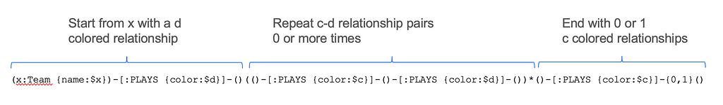
The invert_c_d_path Python below includes the full Cypher query to find the path and invert the relationships:

def invert_c_d_path(x, c, d):
    _, summary, _ = driver.execute_query("""
        MATCH p=(x:Team {name:$x})-[:PLAYS {color:$d}]-()(()-[:PLAYS {color:$c}]-()-[:PLAYS {color:$d}]-())*()-[:PLAYS {color:$c}]-{0,1}()
        WITH p ORDER BY length(p) DESC
        LIMIT 1
        FOREACH(rel in relationships(p) |
        SET rel.color = CASE WHEN rel.color = $c THEN $d ELSE $c END)
                                         """,
                                         {"x": x, "c": c, "d":d})
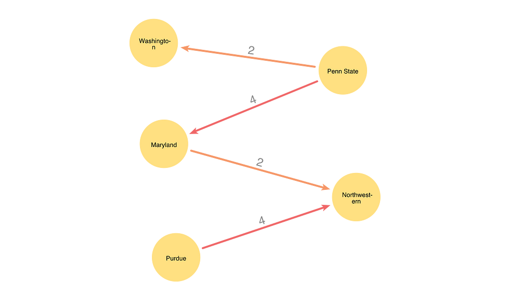
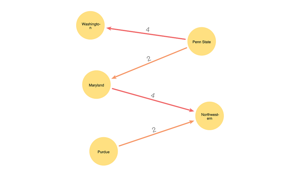
    return summary.counters

After completing the color inversion, the alternating color path starting at Washington now looks like this.

Rotating and Assigning Relationship Colors

The next step of the algorithm is to find a subset of the Vizing fan up to the first node in the fan that has color d free. Because the c-d path recoloring might have changed relationships associated with fan nodes, we can’t rely on the list of incident colors returned by the get_fan_candidates function earlier in the process. The get_rotate_fan function checks the fan nodes until it finds the first one with d free. See the Misra and Gries paper for proof that such a node must exist in the fan.

def get_rotate_fan(fan, d):
    rotate_fan_records, _, _ = driver.execute_query("""
        UNWIND RANGE(0, size($fan)-1) AS idx
        MATCH (g:Team {name:$fan[idx]})
        WHERE NOT EXISTS {(g)-[:PLAYS {color:$d}]-()}
        WITH idx LIMIT 1
        RETURN $fan[..idx + 1] AS rotateFan
                                                    """,
                                                    {"fan":fan,
                                                     "d":d})
    record = rotate_fan_records[0]
    return record['rotateFan']

In our example, d = 2, and Michigan already has a 2-colored relationship. We continue checking the next node in the fan and find that Oregon has 2 free, so the get_rotate_fan function returns [‘Michigan’, ‘Oregon’].

The final step is to rotate the colors assigned to the relationships in the rotation fan. The first relationship in the fan is the uncolored relationship r. We assign that relationship the color of the second relationship in the rotation fan. Each subsequent relationship in the rotation fan is assigned the color of the following relationship. The last relationship in the fan is assigned color d. We know that color d is free on the last relationship of the rotation fan because we selected the rotation fan to meet that condition.

def rotate_and_assign(x, fan, d):
    _, summary, _ = driver.execute_query("""
        MATCH (g:Team {name:$x})
        UNWIND $fan AS f
        MATCH (g)-[r:PLAYS]-(:Team {name:f})
        WITH collect(r) AS rels
        OPTIONAL CALL (rels) {
        UNWIND range(0, size(rels)-2) AS i
        WITH rels[i] AS rel, rels[i+1]['color'] AS color
        SET rel.color = color} 
        WITH rels[-1] AS w
        LIMIT 1
        SET w.color = $d
    """, {"x":x, "fan":fan, "d":d})
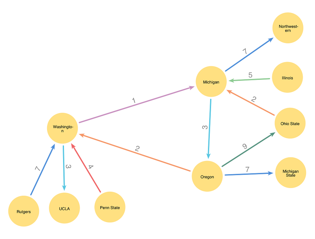
    return summary.counters

The image below shows the result of this iteration, with Washington-Michigan assigned color 1, which was formerly assigned to Washington-Oregon. Washington-Oregon has been assigned color 2, which was the d color selected earlier.

Running the Algorithm for Each Uncolored Relationship

All the steps for a single iteration of the algorithm are contained in the color_relationship function:

def color_relationship(x, f1, colors):
    max_fan, x_incident_colors = get_maximal_fan(x, f1)
    c, d, inversion_required = choose_c_d(max_fan, x_incident_colors, colors)
    if inversion_required:
       invert_c_d_path(x, c, d)
       rotate_fan = get_rotate_fan([fe['name'] for fe in max_fan], d)    
    else:
        rotate_fan = [fe['name'] for fe in max_fan]
    rotate_and_assign(x, rotate_fan, d)

Call the color_relationship function for each uncolored relationship in the graph to obtain a fully colored graph similar to the one shown at the beginning of this article.

After completing the coloring, you can run the validate_coloring function to verify that no node has more than one relationship of the same color:

def validate_coloring():
    records, _, _ = driver.execute_query("""
        MATCH (g:Team)-[b:PLAYS]-()
        WHERE b.color IS NOT NULL
        WITH g, b.color AS color, count(*) as colorCount
        RETURN max(colorCount) AS maxColorsPerNode""")
    print(f"max colors per node {records[0]['maxColorsPerNode']}")
    assert records[0]['maxColorsPerNode'] in [None, 1], "Coloring is invalid"

Going Further

I hope you’ll be able to apply relationship coloring to your own problems where multiple entities interact but must interact one at a time. Beyond sports scheduling, relationship coloring has applications in production process scheduling and network communications. Relationship coloring can be extended to multi-graphs, where pairs of nodes can have more than one relationship between them. Jeffrey M. Gilbert covers the topic in his article “Strategies for Multigraph Edge Coloring.” Relationship coloring is also a key concept in the Neo4j Parallel Spark loader. Using Neo4j to track graph states and find paths in the graph makes solving these relationship coloring problems more manageable.

---

Solve Scheduling Problems With Relationship Coloring and Neo4j was originally published in Neo4j Developer Blog on Medium, where people are continuing the conversation by highlighting and responding to this story.