GeneWeaver: Building a Graph to Map Variants to Genes Using Neo4j 4.x and Bulk Import
11 min read

Editor’s note: This presentation was given by Matthew Gerring at NODES 2021.

The organization I work for, Jackson Laboratory, is a nonprofit biomedical research institution discovering precise genomic solutions for diseases and empowering the global biomedical community in the shared quest to improve human health. Our researchers at JAX are studying genetic backgrounds associated with cancer, Alzheimer’s, and addiction. The graph work that I will be describing was published in Nature by my colleagues: Tim Reynolds, Jason Bubier, Elissa Chesler, and Erich Baker.

I will start by pointing out the mouse and human in the model above. It could be a human with technically any other species, but at JAX we are focused on mice and how they link to humans. So if you look at disease in mice, you can make inferences about humans, and vice versa. In my team’s research paper, they pointed out that much of this data used to find links could be in a graph form. However, the data exists in many different file formats, as seen in the upper half of the diagram. This brings me to Neo4j.
What Is the Data?
What I’ll be covering in this post is how we got the data into the “brains” of Neo4j. First of all, what is the data? In the case of human beings, it is around 100 gigabytes of files in different zipped up text formats. I’ll show how that data is made available to researchers.
The input files are lots of zipped up text tables separated by a character, such as a comma, a space, or a tab. Also, each row in the data can include a list separated by a semi colon. With hundreds of gigabytes of data to run through, the problem is capturing all of this information in one structure.
Why Did We Choose a Graph?
Taking a step back from the problem of sorting through large amounts of data, why would we look at graph, apart from the fact that the researchers draw graphs when they talk about this data? We need to be able to ingest data of this size reasonably quickly. All of the technologies that you might compare to graph are going to be able to do that, but once we have this data, we want to really talk to it in a graph format, which could be with GraphQL or Cypher. We just need a successful graph query language that’s also equally efficient for tree-shaped data.
SQL databases would be slow querying our data because our data is tree-shaped. Also, we don’t want to have join tables at different points; we want to be able to traverse our connections directly. Finally, we want to ingest new data efficiently. This can involve complex nodes and edges interacting with existing data, meaning we need a graph database to solve this problem.
Why Did We Choose Neo4j?
This leads me to why we chose Neo4j. First, when we imported our data, it came out as roughly a billion nodes and 10 billion relationships, and Neo4j easily scales to this.
Second, Neo4j has a REST API, which allows us to send Cypher queries to an endpoint and get back a table. So that means we can have a shell script or something with a curl command that a researcher can push in a prototype graph. Very often, researchers will have input files with hundreds of thousands of gene variants and want to get a table back. That’s where Neo4j’s REST API is perfect for our use case.
Another key thing about Neo4j is the APOC functionality, which is very useful for us when analyzing tissues with our graph. We’re also interested in the machine learning Neo4j has.
First Graph Prototype
An earlier graph prototype we had was based around a SQL database. It reads all of our data into memory because you’re not really doing biology properly unless you read everything into memory and use a supercomputer. This was then written out to tables, which gives most of the functionality of the graph by having queries that can be called from it.
An issue with the prototype was reproducibility. People are always experimenting and producing new input data and we reckon that every four months we would need to rebuild this graph entirely. We would basically have to throw away the old one and download all the new data and rebuild the graph because science is moving forward that quickly. So any successful graph that we built would have to be automated.
Second Graph Prototype
My colleague at JAX, Jake Emerson, made another prototype based in Python, which streamed the data from these input files and used transactions. This became a good basis for what we later accomplished, which was to speed up building this graph in a reproducible way.
Increased Ingest Speed for Graph
I played around with Jake’s code and swapped it over from Python to Neo4j and used OGM. Let’s say you have a gene in the file, and then you have a few transcripts and they link back to the genes somehow. This means the file has multiple entities: nodes and relationships within a flat table. To stream those objects and create the graph, we used transactions, which took around eight or nine milliseconds per node. That time was based on our benchmark of 1.7 million nodes. So the time for the full graph being built would be about 100 days, which means we can only do three a year. That was way too slow. So I moved to Java and brought it down to 57 days, but obviously that’s still too slow.
So then I committed it based on transactions and that halved it again. I then used multiple threads and a chunked read because these files are organized to have the gene followed by the transcripts belonging to the gene. You can actually optimize around this organization and read a whole gene chunk, which speeds up the building of the graph. I got it down to two or three days at this point, which isn’t terrible. However, another colleague was using Neo4j in another project and asked, “Do you know about bulk import?” I didn’t.
My colleague went on to explain to me that there was this bulk import feature and that, rather embarrassingly, I’d spend time optimizing something when there was already a way of doing this. It did turn out that some of our fast transactions will be needed later for updates in the graph, but moving over to bulk import just takes a single thread and pauses these import files and writes output files. Bulk import took down the building of the graph to half a day or a day. This meant I could run it and have a graph the very next day.
Streaming Data
We didn’t want to hold the data in memory as we’d done with the earlier prototypes. Instead, we wanted to stream the data. There are packages for streaming data, but I wanted the most efficient stream for this use case in order to get the times down. I wrote an IO package for some existing file formats which have readers in Java but are not optimized. So, I streamed from the files using Java streams and mapped between those.
Bulk Import
What does the bulk import look like? It is a command line interface: you log into where you want to build it, have Neo4j available, and then download the data. Then you run the command line interface to build the files. It’s not as straightforward as directly transforming data because it is too large to fit in memory, but the database caches the files as you’re writing them so you can create the correct links. Neo4j has a fantastic tutorial online for bulk import, and I encourage anyone who is thinking of using bulk import to go and have a look at that.

Our use cases stretched a little bit in that it is continually rebuilding quite large data, but it’s still much smaller than many social networks and perfectly doable. One other thing to note is that when we were building these files that Neo4j uses for bulk importing, at least for our use case, Neo4j 4 was quite a bit faster than Neo4j 3.
Mapping Genes and Connections
With bulk import, you stream objects and then map them, but it’s not quite as simple as that because multiple objects come out. Those objects then have connections, for which you need to write the connection files for those objects. The stream of objects coming from a single file is then connected using a flat map.
For example, if you imagine a gene object comes out of this file in Java, that gene object will then have connections, which will be multiple objects or relationships to other objects. It goes from a stream of genes to a stream of genes plus the connections. In fact, the original stream is heterogeneous, so it might see a transcript and then map back to the gene. It might need to go the other way, but all of these entities are coming out in a stream and then saved to their individual bulk files. In some cases, a database is written so that there are different tables, some around a few gigabytes and others only a few megabytes.
Deployment
Once we’ve managed to take all these input files and build them into the files that Neo4j can slurp up, how do we actually deploy that? What does it look like for users to use it?
We have a bit of an unusual use case, in that we have a low number of users doing a large number of queries. For instance, one user may import a CSV file looking at 100,000 variants. That might be one interaction using the database, and then for a few days, we might have no one using it. That’s a bit different to other cases where it’s intensively used by more users. So we looked into AuraDB which is the Neo4j cloud offering, but for our use case, it’s not the best fit. It’s designed more for concurrent users, whereas we don’t have that many users.
So we looked into starting a Community Edition instance on Compute Engine. That worked out okay, so we installed Neo4j on a Compute Engine VM and then used Google Storage. On Google Storage, we could download all those data files, build the graph using the commands I’ve discussed, and import it. Then we had all the data files and the complete graph. Now we can interact with the graph.
What Does Our Graph Look Like Today?
Today, there are around 3.6 billion relationships between genes, transcripts, variants, eQTLs, and data from different sources that map between genes. For a given mouse gene, we look at the homologs and orthologs and the links between the mouse and another species.

Primarily, we are of course interested in humans and their links. I’ve been importing them with different tags so that you can actually traverse the graph and then ignore the orthologs between genes that you might not agree with as a researcher. We’ve been adding links between various variants and mouse genes by parsing through the data that our institution produces. All in all, the graph is around the scale of a billion nodes, which is not unmanageable.
What Does Using This Graph Look Like for a Researcher?
Just going on to a few examples, if you’re a researcher, the graph wouldn’t look like a front end in particular. It is available to people to bring up the excellent Neo4j GUI and try out different maps through these genes, but the graph is relatively simple.
With these eQTL links, there might be scores between one gene and its variants. So you’re not actually traversing into a deep graph, but what you are doing as a researcher is firing off lots of variants at this graph and trying to build up what those individual relationships would be. You might have a gene set of known variants that are associated with disease and want to look at that through the known links in another species. You might want to go from a mouse into a human; you’ve got some variants that you think are associated with disease, and you want to know what mice to look at or what variants should be in those mice.
For the following examples, the interface is a curl command, which we actually execute on the database.
Example 1: Table of Links Between Genes
MATCH (h:Gene {species: ‘Homo sapiens’}) -- (m:Gene {species:’Mus musculus’}) RETURN h.geneName,h.geneId,m.geneId,m.geneName;
This first example is saying for two species, give me a table of all the links between them. We could actually pare that down if a researcher only believed in homology as a link.
Example 2: Table of Human Genes Getting Chromosomes, Start to End
MATCH (g:Gene {species: ‘Homo sapiens’}) RETURN g.geneId,g.geneName,g.chr,g.start,g.end LIMIT 25;
This second example is replacing the need to get the files and parse them. It’s not even really using the graph. Instead, it’s just saying for all homosapien genes, give me the start and end position of the chromosome and the start and end position of that gene on the genome. It replaces the need for writing in R or Python to get the table with just running a Cypher Query.
Example 3: Table of Genes Which Are Linked to a Table of Variants in Another Species Without an Ortholog
LOAD CSV WITH HEADERS FROM

“https://bitbucket.org/../variants.csv” as row MATCH (n:Variant ({variantId: row.id})-[e:VARIANT_EFFECT]-(t:Transcript)-[]-(g1:Gene) WHERE NOT (g1)-[:ORTHOLOG]-(:Gene) RETURN n.VariantId,e.sequenceVariant,t.transcriptId,g1.geneId;
The final example is one I’ve already discussed, where we have a bunch of variants in a CSV file. We want to traverse the graph, maybe limit it to certain links between genes, and we want it to return a table of genes.
Upcoming Work
We are continuing to add the data sources.
Next, we want to integrate the Neo4j graph with geneweaver.org. Geneweaver.org already allows you to build gene sets for effects of diseases, and the next step would be the ability to put that gene set into the graph and get a table of the relationships that the graph thinks exists.
We can also do further analysis based on tissues using APOC, and we’re thinking of deploying this graph externally. At the moment it’s a Google Cloud deployment, but that’s not public, though we could potentially make that available to other researchers around the U.S and the world. At that point, we would need to go back and look at Neo4j Aura if it becomes wildly successful.
Conclusion
In conclusion, Neo4j scales well beyond our requirements. The graph approach makes queries easy for science. The REST API is extremely useful and something we use all the time. If you use indices, which we use often to make our queries faster, then you’re going to need the disk space. Several terabytes in our cases is not huge. We think that this has great potential. I should probably point out that our solution is actually beta, although Neo4j is a production system of course. So we haven’t done scientific level tests to check that all of the data has been ingested and put into the graph correctly.
Finally, I want to thank Robyn Ball, Erich Baker, Jason Bubier, Elissa Chesler, Jake Emerson, Howard, Tim Reynolds, everybody in the IT departments of the two institutions that are collaborating, thanks a lot to Neo4j because they helped me with support questions, and thanks to other members of the GeneWeaver team who got me working with things like Maven central.
Share Article


Explore
Related Articles

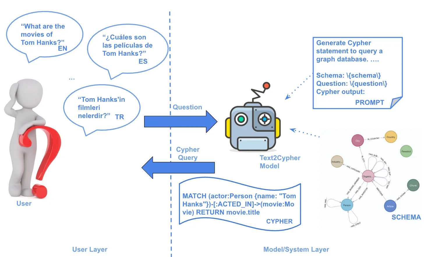
Text2Cypher Across Languages: Evaluating Foundational Models Beyond English