Graph algorithms for community detection & recommendations


19 min read

Editor’s Note: This presentation was given by Mark Needham and Amy Hodler at NODES 2019 in October 2019.
Presentation summary
Our names are Mark Needham and Amy Hodler. Mark works on the Neo4j Labs team, which is a team that helps Neo4j integrate with different technologies and explores different areas where people might be interested in applying graphs. Amy works on Analytics and AI Programs.
In this post, we will talk about graph algorithms for community detection and recommendations, and further understand how to actually employ various graph algorithms. Particularly, we’ll look at Twitter’s social graph, view its influencers and identify its communities.
We’ll also provide in-depth explanations of the following Centrality algorithms:
Near the end, we’ll look at community detection algorithms like the Louvain Modularity algorithm, which helps us evaluate how our groups are clustered or partitioned.
Full presentation: Graph algorithms for community detection & recommendations
One of the first questions we get is: What are graph algorithms and analytics, and why would we use them?
Let’s first do a quick comparison between queries and graph algorithms:

You’re probably familiar with queries, where you have something specific that you’re trying to look for or match a pattern with. In such cases, you know what you’re looking for and are trying to make a local decision. Queries can answer questions like “How many people four hops out from this person have a similar phone number?”
With graph algorithms, we’re usually looking at something more global and conducting some form of analysis. It’s often an iterative approach, where you’re learning based on the overall structure or topology of the network.
Another question many users have is when graph algorithms are not the right fit or process to utilize. If you want to find something with just a few connections and it’s very specific or involves basic statistics (i.e. an average ratio), graph algorithms might not be the right path to take.
Another example of when you wouldn’t use graph algorithms is for regular reporting processes, such as sales summary reporting, which are already very defined and well-organized.
What do people do with graph algorithms?
There are three things people generally do with graph algorithms, and they all have to do with trying to understand and predict more complex behavior.

First, we have propagation pathways. This concerns how we visualize the ways in which things spread through a network. Maybe we’re talking about a rumor or a disease, where we want to understand the paths they take.
Second, we have flow and dynamics, which is also about how things move, but more about its flow. What’s the capacity of my network? How much telco traffic can I route on my network? If I have a router that goes down, what’s the secondary pass that we might take?
The third area people generally look at is understanding the dynamics of groups, including interactions between different communities and their resiliency. Is my group likely to stick together? Are they likely to fall apart?
Ultimately, what’s in common between these three areas is that you’re really trying to understand relationships and structures.
Using graph algorithms
So how do I actually employ graph algorithms? There are two main major areas:
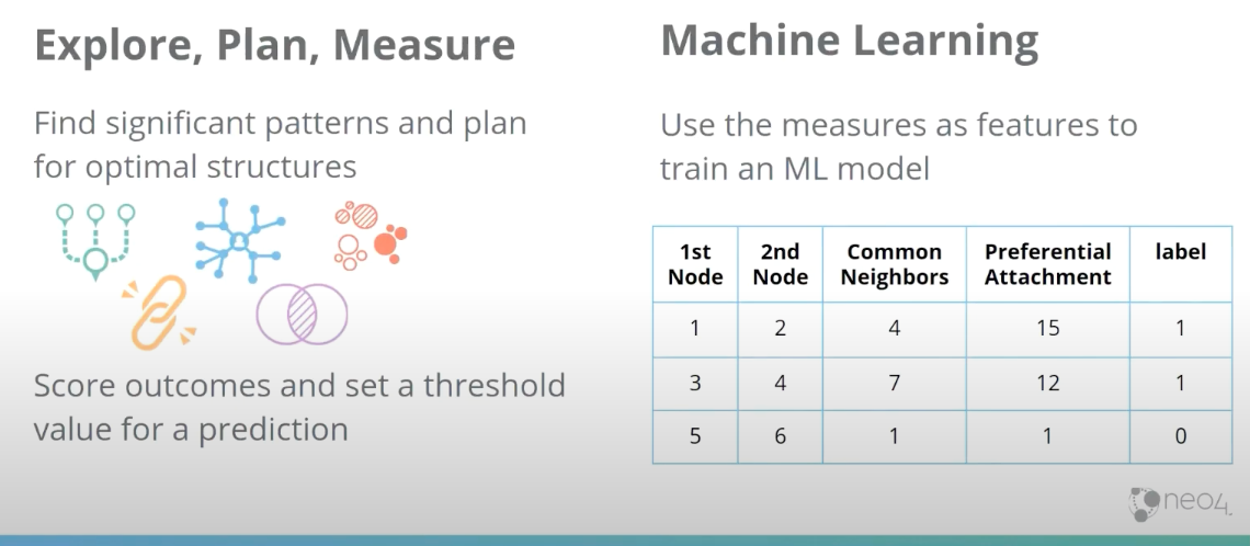
One area is the analysis itself, where you’re exploring your graph, finding patterns or looking for some kind of structure. You can set a threshold for these measures and make a general assumption or prediction.
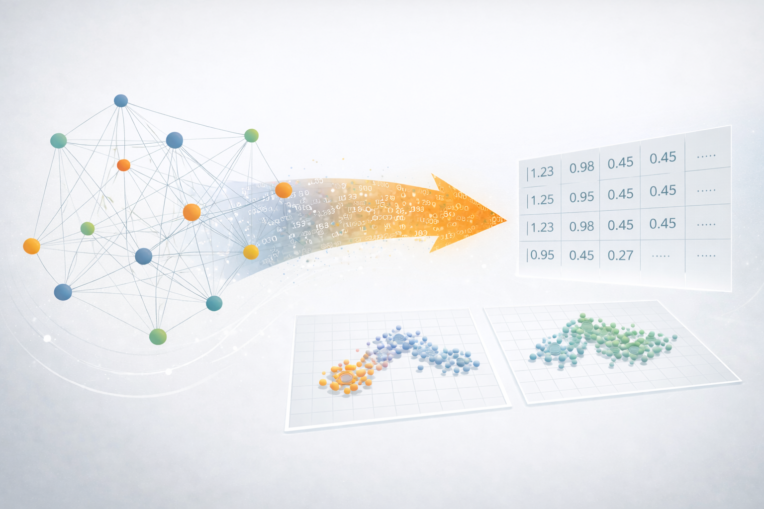
The other area that’s becoming really popular right now is machine learning. Here, users usually start with a set of graph algorithms, run them, come up with a metric and conduct an extraction of that metric into a table or a vector. From there, you can run machine learning on it.
Neo4j graph algorithms library
We’ve got quite a few algorithms in the Neo4j Graph Data Science Library. If you haven’t yet read the Graph Algorithms book, it’s a great way to get started on it. You can get a free download online.
In the library, we have over 45 graph algorithms. We keep updating that number because every time we turn around, our team has added more. But, these algorithms generally fall into the following five categories:
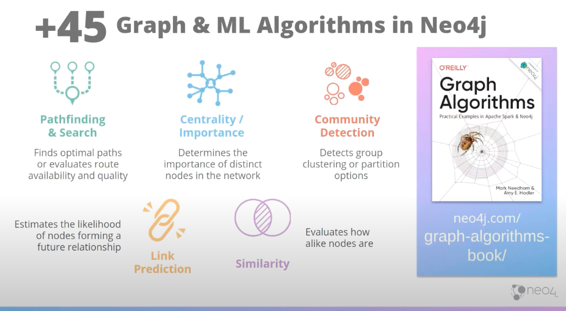
- Pathfinding tells you how to find the optimal route or evaluate the quality of the routes you have.
- Centrality is about finding the important and influential nodes in your network.
- Community detection, or community understanding, informs you about the clusters and partitions within your community. Are they tightly-knit? Am I looking for hierarchical searches?
- Link prediction is an interesting category that’s more focused on nodes themselves. It looks at whether nodes are likely to become connected in the future, or if there’s something that should be connected. This is all based on the topology of the nodes.
- Similarity looks at how alike nodes are based on different factors, whether it’s the attributes of the nodes or the relationships they have.
So how do you actually use and call these algorithms? After you have the library installed, you can call them through a Cypher procedure, then pass in whatever configurations and attributes you might have, what labels you want to use and what parameters you want to set. From there, you have a choice of whether you want to stream the result or write them back to the graph. Note that if you decide to stream them, you could have a lot of results to look through.
Cypher projections
Cypher projections are a really powerful way to work with graphs and algorithms. It basically lets you pass through a Cypher statement to match specific nodes and relationships, and obtain the graph in the shape you need.
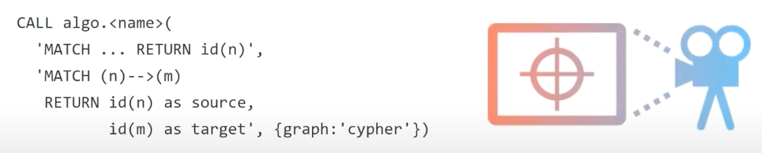
For example, if you want to run an algorithm on a subset of certain people with a particular zip code, you wouldn’t necessarily need to run that on the whole graph.
Inferring relationships: Russia Twitter trolls
Here’s an example of how we can use Cypher projections to infer interesting results. Our developer relations and Neo4j Labs team ran a really nice example involving Russian Twitter trolls, looking at tweets, where they came from, who wrote them and who retweeted them.

We were able to infer relationships using Cypher projections. As you can see here, we have a couple of users on Twitter, as well as a tweet that was posted and retweeted by somebody else. From there, we were able to actually infer the relationship between the first and second Twitter users, even though it’s not a direct relationship.
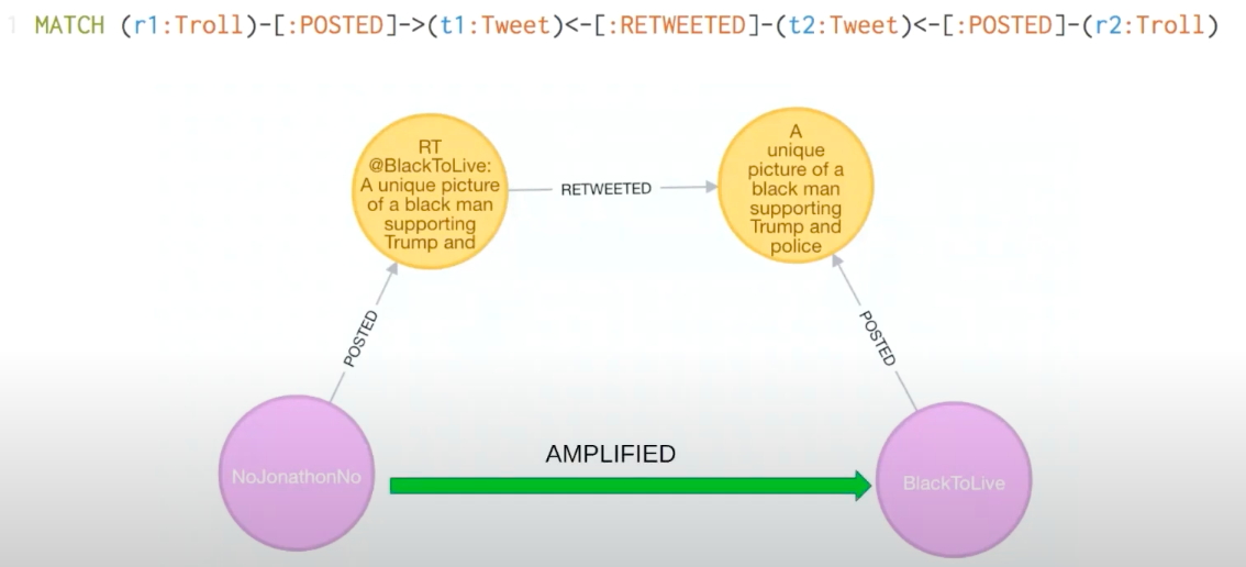
In this way, you can use Cypher projections to infer relationships and run different algorithms on them.
Below is an example of how you can run the PageRank algorithm over that Twitter troll’s graph, where the inferred relationships imply that Troll Two is amplifying Troll One.
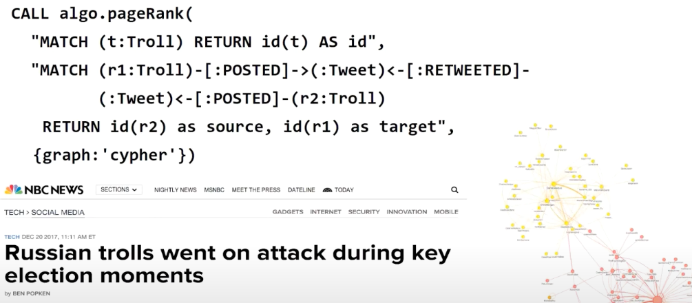
The main idea here is that when you have a relationship that points from you to someone else, it means you’re amplifying; essentially, you’re indicating that this person is credible. That’s what the RETWEETED relationship means here.
In an example later on in this post, we’re actually going to use a more direct amplification, which is that if someone follows the other person, it means they amplify them. If you wanted to, you could even indicate various levels of amplification. For example, following might represent a weak amplification, while retweeting might represent a stronger amplification.
How does it work?
Here’s a quick breakdown of how this works, because it’s not quite the same as what you might be familiar with from the querying approach discussed earlier.
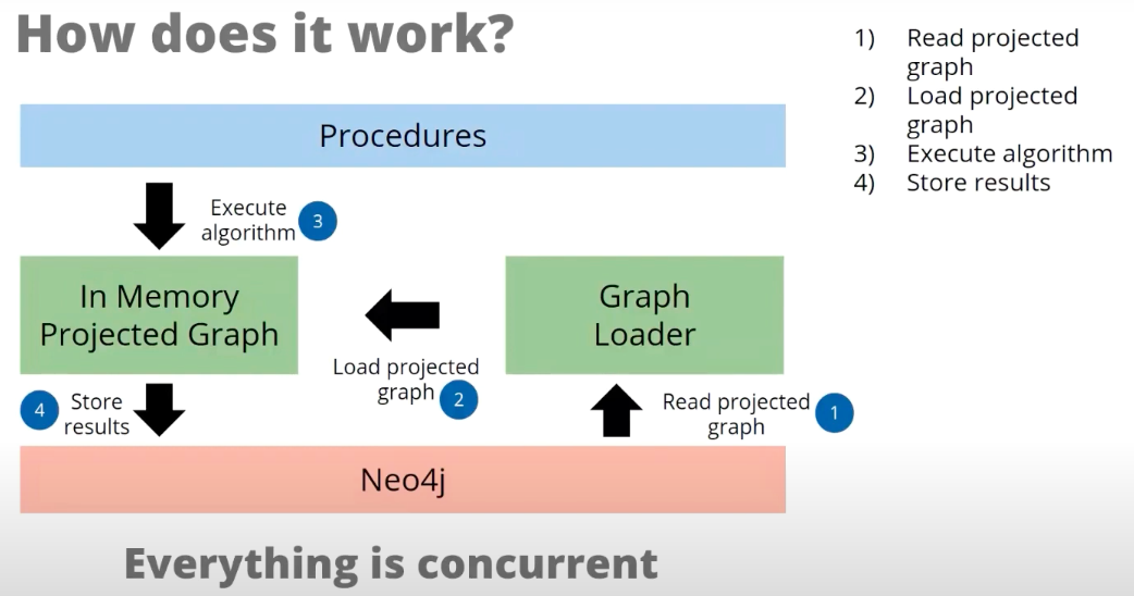
Normally, the process goes a little bit like this: You write your query, and it’s run by the Cypher engine, which runs it against Neo4j, loads some of it into memory while it’s running and sends it back.
But, the model here is actually quite different, and there are two ways you can do it. Generally, the first step involves the graph-loading process, where the projected graph could be the whole graph or a subset of that graph, which could be defined by using a node label, a particular relationship type or a pair of Cypher queries.
From there, we can also choose to run the graph in a mode where it keeps the graph only for the duration of the query and erases it once the query is finished.
The third step is to run the algorithm in a memory-projected graph. These results will either be stored in Neo4j or streamed back to the procedure.
Enter the NEuler
A colleague of ours started up a project called NEuler, which stands for Neo4j Euler (Euler was the creator of graph theory way back when).
Our colleague created a graph app, which is a React application that sits on top of the graph algorithms library and allows you to use these algorithms without having to write any of the Cypher code we just looked at. This is a really good way of getting started, and we consider this app as training wheels for getting started with graph algorithms.
If you want to install it yourself, you can get it on install.graphapp.io. This is the Graph Apps gallery, where you can do a one-click install of different graph apps that have been either written or curated by the Neo4j Labs team.

As you can see in the first row, the third item is the Neo4j Graph Algorithms Playground.
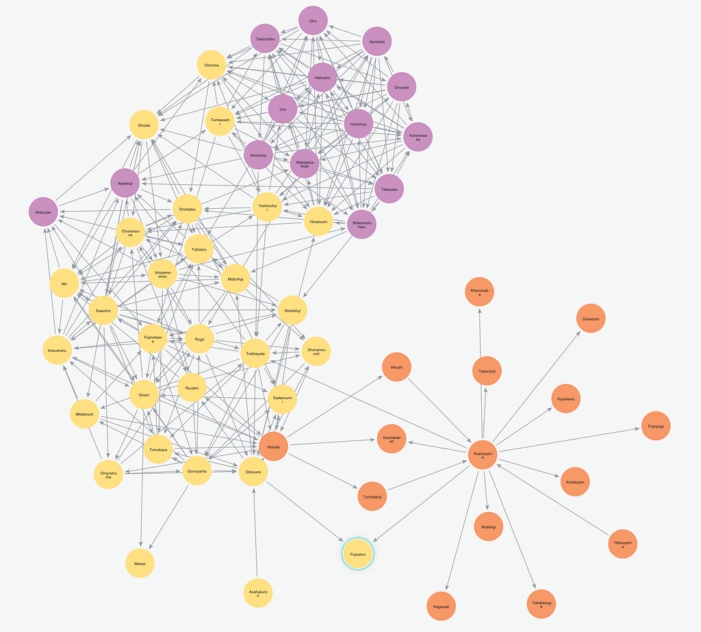
Investigating the Neo4j social graph
We’ve actually created a graph of the Neo4j Twitter Graph:

We scraped all the tweets from the past nine months with the Neo4j and graph database hashtags. Then, we looked at the users who wrote those tweets and obtained their follower and friends graphs.
At the moment, we haven’t pulled in the retweets as we did in the Twitter trolls example, so we’re just going to focus on the followers graph for this talk and see what we can discover about this graph community.
To do this, we’re using a tool called Twint. The official Twitter API has strict rate limiting, as they don’t want users extracting that followers graph. But, it’s really interesting for graph analytics, so we’re using this scraping tool to obtain the data and then we’re going to use NEuler to explore it.
If you can’t be bothered with the scraping step, we’ve actually created it as a sample graph in NEuler. In this post, we’ll use the Twitter one I curated, but there are two other ones, one of which contains European roads and the links between them, and the other of which includes interactions from the Game of Thrones television series. All three of these are really interesting for quickly doing a graph analytics-type workup.
Now let’s discuss what types of analyses we can conduct.
Centrality algorithms
There four main types of Centrality people typically look at, and we’re going to look at three of the four in a little more detail. They’re quite nuanced in how they interpret what influence means.

For example, Degree looks at the number of connections somebody has; in the upper left of the image above, A has a high degree with a lot of connections. Closeness, on the other hand, looks at how quickly a node reaches other nodes. Betweenness looks at the influence each node has over the flow of resources, flow of information and potential bottlenecks. PageRank, of course, looks at overall influence and isn’t necessarily based on the number of connections.
Degree centrality
Let’s first look at Degree Centrality. As we discussed earlier, this measures the number of direct relationships by looking at in-degrees. In the image below, for example, someone with no relationships going into them is labeled 0, while someone labeled 6 has six relationships coming into them.

Degree Centrality is probably the simplest of the Centrality algorithms. With it, you can look at in-degree if you’re interested in popularity, and out-degree if you’re interested in gregariousness. You can also globally average them to analyze how connected your overall graph is.
However, it’s important to realize that if you’ve got supernodes or lumpy distributions of relationships, it will skew your overall results. Other algorithms are probably better for influence over more than just direct neighbors.
Now, when would you use this? One example is to look at the likelihood of somebody having the flu. If I have a lot of friends, I’m more likely to get the flu if the people within my network have the flu. In this way, you can understand a lot about immediate and fast types of connections. And as we discussed earlier, you can also do a quick estimation of your network to look at minimums, maximums and mean degrees.
People who aren’t really into graphs might use this one first. When people talk about Twitter analysis, they mostly think that people who have the most followers also have the most influence. But, as we’ll see from the next few algorithms, there could be people who have less direct followers but more influence in slightly different ways.
PageRank
As we saw just now, Degree is a very direct measure of influence. PageRank, on the other hand, shows how to look at the influence of nodes in consideration of their neighbors, connections, their importance and the influence each one of those neighbors has, which makes it more iterative.

Here’s an analogy that might help you understand PageRank more clearly: A foot soldier who has a lot of friends is not as high up as a foot soldier at the same rank who happens to be friends with the general. In this way, each friend’s influence or ranking impacts how influential they are.
One tip on PageRank is that you can set dampening factors, which change how quickly you jump to other nodes so you don’t end up in a dead-end. The defaults are set for a power-law distribution, a situation in which you have hubs and spokes. However, if your data doesn’t distribute that way, you can play around with various dampening factors.
The other thing to be careful about is mixing node types, as PageRank assumes a single node type. For example, looking at the influence of a human versus a restaurant doesn’t really make sense, because you’re ranking a person against a business.
Also, keep in mind that the relationship type implies that you’re giving some credibility or amplifying the node you’re pointing to. If this isn’t the case, you’ll get a fairly nonsensical result from running this algorithm.
Let’s take a look at when you might use PageRank. There are a lot of domain-specific variants of PageRank, such as Personalized PageRank, which means that every time you hop, you go back to either a particular node or a set of nodes. This is used in very interesting ways, such as personalized recommendations. For example, Twitter uses a Personalized PageRank to recommend who to follow.
The other thing to keep in mind is that it’s a rank. The actual score isn’t as meaningful as what’s on top, what’s second, what’s fourth or what’s 10th.
Betweenness centrality
Betweenness is a lot of fun. Basically, it’s a measure of the sum of percentages or shortest paths through a node. For example, the A node here in the middle has the highest Betweenness Centrality, which essentially looks at bridges between communities.

This can be a very computationally heavy algorithm if you’re running it in its original form, as you have to look at every path, understand the shortest paths and calculate based on that. This is why we use approximations – such as the RA Brandes approximation – in large graphs. You might also want to pare down so you’re not looking at the Betweenness Centrality of everything, but rather just specific products, particular components in your products, people in your network or how you’re routing packets in an IT network.
Moreover, Betweenness Centrality assumes communications happen between nodes along the shortest paths, though this isn’t necessarily the case in actual real life. This is just something to think about: Are my communications and routing actually going along the shortest and most efficient paths?
Let’s look at a couple of use cases with Betweenness Centrality. As you can see below, with Betweenness Centrality, you can identify bridges and find bottlenecks, vulnerabilities and control points.
The example here was an evaluation done with a country’s electric grid, particularly looking at rippling and cascading failures they were having in their electrical grid. They thought that if they added more redundancy, cascading failures would go down and resiliency would go up.
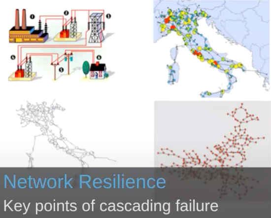
However, when they looked at it as a graph and analyzed where the vulnerabilities were, they realized that if they actually removed some of the control points or communications between the grid, their resiliency would actually go up. This makes sense when you imagine failures spreading like a disease; they were actually providing too many routes for those failures to propagate widely.
Community detection algorithms
Community Detection algorithms help us to evaluate how our group is clustered or partitioned. Naturally, the next thing that we’re interested in is what we’re bridging to.
Louvain modularity
For this purpose, we’ll use an algorithm called the Louvain Modularity algorithm, which is one of many modularity algorithms. Again, it doesn’t do brute-force modularity computation but rather partakes in an approximation approach. The main idea is that it puts nodes into communities and then scores the communities based on how closely connected nodes are within the community versus how well they’re connected outside. In this way, you’re almost trying to find the ratio between those two things, where you want nodes in the community that are more tightly connected inside than they are outside.
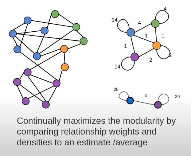
Again, you’ll never get a perfect result, as it’s an approximation. It’s also an iterative algorithm; in every iteration, I’m testing whether I can move this node out of that community into another one, and seeing whether that makes things worse or better. Eventually, you’ll get to a point that’s reasonably stable, and those might be the communities you end up with.
One cool feature of this is that after every iteration, you can get it to show you what the community looked like after every iteration, which allows you to see what we call intermediate communities.
For example, after a single iteration, you might see a few smaller communities. But, as iterations go by, they might end up being merged into larger ones. In the end, you might end up with just 10 communities, but if you want to know the breakdown of those smaller ones inside the 10, you can look back at the intermediate communities that were computed along the way.
Regarding use cases, we can use this algorithm to find communities and large networks and evaluate various grouping thresholds. Moreover, one of the interesting aspects of looking at fraud or any kind of network with Louvain is that because you get the intermediary categories or groups, you have the ability to control how tightly you want that community to be defined.
Essentially, you can set a threshold to say, “Is this somebody who’s just not behaving well,” or “Is this perhaps a really tight community that we need to look at as a potential fraud ring?”
What do we do with this? How would we make recommendations using these algorithms?
Targeting recommendations
Let’s say you want to do recommendations, or you have a distribution or an offer you make to particular people. There’s a couple of different ways you could do that:

The first algorithm we talked about, Degree Centrality, might be used if you want to get an immediate message out to the most people in that community.
The second algorithm looks at overall influence, and PageRank was this example. In this case, I’m looking at the influencer with the broadest reach to the biggest number of people, and maybe takes a little longer to propagate. We might want a ripple effect that’s not as time-critical. In this case, TechCrunch had the highest PageRank.
The third example here looks at communities. This is when we had different promotions, tweets and offers to various sub-communities – maybe the Spring community, versus the Microsoft community, versus a data science community. With these different communities, I’ll want to use different words and offer different things.
The fourth one, Betweenness Centrality, uses those bridges. I want to find a person who has a lot of influence but can help me get my information, or target the specific sub-community I’m interested in.
Learn more
To wrap up, we have a few resources for you. We’ve built a couple of online training courses with slightly different focuses. The first one is about Applied Graph Algorithms, where you build a web application while using graph algorithms to enhance the application and make better recommendations or suggestions to the users. It’s based on the Yelp dataset.
Then, we have the Data Science with Neo4j course. At the beginning of the post, we talked about two different uses for graph algorithms: you can use them directly, or you can use them as part of a data science and machine learning workflow. This course looks at the latter and takes us through some of the steps of how you might do graph data science.
If you’re interested in learning more about how to do this in a hands-on way, I’d encourage you to take a look at these online training courses.
Of course, it would be remiss of us to write a post without mentioning that we wrote a book on this topic. If this is intriguing to you, don’t forget to take a look at it below.
Download your free copy of Graph Algorithms: Practical Examples in Apache Spark and Neo4j.
Share Article


Explore
Related Articles

Neo4j Named “One to Watch” in Snowflake’s 2026 Modern Marketing Data Stack Report

SumoDB in Neo4j: Chaining Multiple Graph Algorithms in Snowflake — Part 3