Graph algorithms in Neo4j: Shortest path


4 min read
Graph algorithms provide the means to understand, model and predict complicated
dynamics such as the flow of resources or information, the pathways through which
contagions or network failures spread, and the influences on and resiliency of groups.
This blog series is designed to help you better leverage graph analytics and graph algorithms so you can effectively innovate and develop intelligent solutions faster.

Last week we looked at the Neo4j Graph Algorithms library and how it is used on your connected data to gain new insights more easily within Neo4j.
This week we begin our exploration of pathfinding and graph search algorithms.
These algorithms start at a node and expand relationships until the destination has been reached. Pathfinding algorithms do this while trying to find the cheapest path in terms of number of hops or weight whereas search algorithms will find a path that might not be the shortest.
We’ll start with the Shortest Path algorithm, which calculates the shortest weighted path between a pair of nodes.
About shortest path
Shortest Path is used for finding directions between physical locations, such as driving directions. It’s also used to find the degrees of separations between people in social networks as well as their mutual connections.
The Shortest Path algorithm calculates the shortest (weighted) path between a pair of nodes.
In this category, Dijkstra’s algorithm is the most well known. It is a real-time graph algorithm, and is used as part of the normal user flow in a web or mobile application.
Pathfinding has a long history and is considered to be one of the classical graph problems; it has been researched as far back as the 19th century. It gained prominence in the early 1950s in the context of alternate routing, that is, finding the second shortest route if the shortest route is blocked.
Edsger Dijkstra came up with his algorithm in 1956 while trying to show off the new ARMAC computers. He needed to find a problem and a solution that people not familiar with computing would be able to understand, and he designed what is now known as Dijkstra’s algorithm. He later implemented it for a slightly simplified transportation map of 64 cities in the Netherlands.
When should I use shortest path?
- Finding directions between physical locations. This is the most common usage, and web mapping tools such as Google Maps use the shortest path algorithm, or a variant of it, to provide driving directions.
- Social networks use the algorithm to find the degrees of separation between people. For example, when you view someone’s profile on LinkedIn, it will indicate how many people separate you in the connections graph, as well as listing your mutual connections.
TIP: Dijkstra does not support negative weights. The algorithm assumes that adding a relationship to a path can never make a path shorter – an invariant that would be violated with negative weights.
Shortest path example
Let’s calculate Shortest Path on a small dataset.
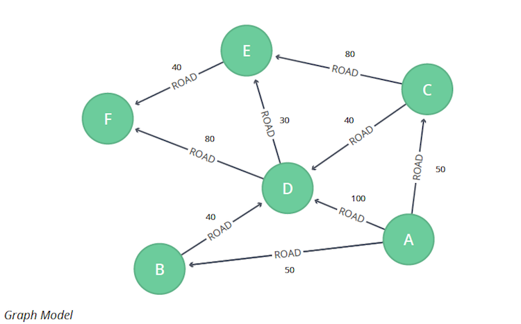
The following Cypher statement creates a sample graph containing locations and connections between them.
MERGE (a:Loc {name:"A"}

MERGE (b:Loc {name:"B"}

MERGE (c:Loc {name:"C"}

MERGE (d:Loc {name:"D"}

MERGE (e:Loc {name:"E"}

MERGE (f:Loc {name:"F"}

MERGE (a)-[:ROAD {cost:50}]->(b)

MERGE (a)-[:ROAD {cost:50}]->(c)

MERGE (a)-[:ROAD {cost:100}]->(d)

MERGE (b)-[:ROAD {cost:40}]->(d)

MERGE (c)-[:ROAD {cost:40}]->(d)

MERGE (c)-[:ROAD {cost:80}]->(e)

MERGE (d)-[:ROAD {cost:30}]->(e)

MERGE (d)-[:ROAD {cost:80}]->(f)

MERGE (e)-[:ROAD {cost:40}]->(f);
Now we can run the Shortest Path algorithm to find the shortest path between A and F.
Execute the following query.
MATCH (start:Loc{name:"A"}), (end:Loc{name:"F"})

CALL algo.shortestPath.stream(start, end, "cost")

YIELD nodeId, cost

MATCH (other:Loc) WHERE id(other) = nodeId

RETURN other.name AS name, cost
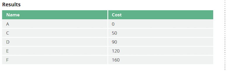
The quickest route takes us from A to F, via C, D, and E, at a total cost of 160:
- First, we go from
AtoC, at a cost of 50. - Then, we go from
CtoD, for an additional 40. - Then, from
DtoE, for an additional 30. - Finally, from
EtoF, for a further 40.
Conclusion
br>
We’ve covered the first in our list of pathfinding algorithms, Shortest Path. Next week we’ll continue our examination of pathfinding algorithms with a look at the Single Shortest Path algorithm, using examples from Neo4j, the world’s leading graph database.
Learn about the power of graph algorithms in the O’Reilly book,
Graph Algorithms: Practical Examples in Apache Spark and Neo4j by the authors of this article. Click below to get your free ebook copy.
Share Article


Explore
Related Articles

SumoDB in Neo4j: Chaining Multiple Graph Algorithms in Snowflake — Part 3


Why machines need embeddings: Turning graph structure into features