Graph algorithms in Neo4j: Single source shortest path


3 min read
Graph algorithms provide the means to understand, model and predict complicated
dynamics such as the flow of resources or information, the pathways through which
contagions or network failures spread, and the influences on and resiliency of groups.
This blog series is designed to help you better utilize graph analytics and graph algorithms so you can effectively innovate and develop intelligent solutions faster using a graph database.
Last week we began our look at pathfinding and graph search algorithms, starting with the Shortest Path algorithm. This week we’ll look at the Single Source Shortest Path algorithm, which calculates a path between a node and all other nodes whose summed value (weight of relationships such as cost, distance, time or capacity) to all other nodes is minimal.

Single Source Shortest Path is faster than Shortest Path and is used for the same types of problems. It is also essential in logical routing such as telephone call routing.
About single source shortest path
The Single Source Shortest Path (SSSP) algorithm calculates the shortest (weighted) path from a node to all other nodes in the graph.
SSSP came into prominence at the same time as the Shortest Path algorithm and Dijkstra’s algorithm acts as an implementation for both problems.
Neo4j implements a variation of SSSP, the delta-stepping algorithm. The delta-stepping algorithm outperforms Dijkstra’s and efficiently works in sequential and parallel settings for many types of graphs.
When should I use single source shortest path?
Open Shortest Path First is a routing protocol for IP networks. It uses Dijkstra’s algorithm to help detect changes in topology, such as link failures, and come up with a new routing structure in seconds.
TIP: Delta-stepping does not support negative weights. The algorithm assumes that adding a relationship to a path never makes a path shorter – an invariant that would be violated with negative weights.
Single source shortest path example
Let’s calculate Single Source Shortest Path on a small dataset.
The following Cypher statement creates a sample graph containing locations and connections between them.
MERGE (a:Loc {name:"A"})

MERGE (b:Loc {name:"B"})

MERGE (c:Loc {name:"C"})

MERGE (d:Loc {name:"D"})

MERGE (e:Loc {name:"E"})

MERGE (f:Loc {name:"F"})

MERGE (a)-[:ROAD {cost:50}]->(b)

MERGE (a)-[:ROAD {cost:50}]->(c)

MERGE (a)-[:ROAD {cost:100}]->(d)

MERGE (b)-[:ROAD {cost:40}]->(d)

MERGE (c)-[:ROAD {cost:40}]->(d)

MERGE (c)-[:ROAD {cost:80}]->(e)

MERGE (d)-[:ROAD {cost:30}]->(e)

MERGE (d)-[:ROAD {cost:80}]->(f)

MERGE (e)-[:ROAD {cost:40}]->(f);

Now we can run the Single Source Shortest Path algorithm to find the shortest path between A and all other nodes. Execute the following query.
MATCH (n:Loc {name:"A"})

CALL algo.shortestPath.deltaStepping.stream(n, "cost", 3.0

YIELD nodeId, distance

MATCH (destination) WHERE id(destination) = nodeId

RETURN destination.name AS destination, distance

The above table shows the cost of going from A to each of the other nodes, including itself at a cost of 0.
Conclusion
We’ve covered the second in our list of pathfinding algorithms, Single Source Shortest Path. Next week we’ll have a look at another pathfinding algorithm, All Pairs Shortest Path, which calculates the shortest (weighted) path between all pairs of nodes.
Learn about the power of graph algorithms in the O’Reilly book,
Graph Algorithms: Practical Examples in Apache Spark and Neo4j by the authors of this article. Click below to get your free ebook copy.
Share Article


Explore
Related Articles
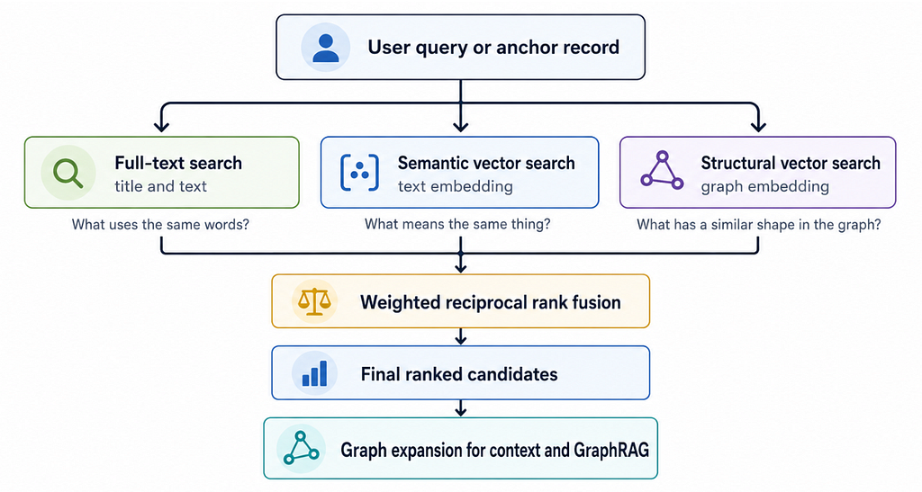
Hybrid Search in Neo4j: Full-Text, Vectors, and Graph Topology with Cypher

Neo4j Named “One to Watch” in Snowflake’s 2026 Modern Marketing Data Stack Report

SumoDB in Neo4j: Chaining Multiple Graph Algorithms in Snowflake — Part 3