Graph Databases for Beginners: Graph Search Algorithm Basics

When he wasn’t busy shelving books, collecting overdue fines and shushing children (we can only presume) in the library at the House of Wisdom, Muhammad ibn Musa al-Khwarizmi was also keeping up a few other side projects: inventing algebra, popularizing the Hindu-Arabic numeral system in the West, helping Islamic astronomy turn a new corner and putting Ptolemy to shame with an updated list of the coordinates of about 2402 places on earth. He probably couldn’t imagine that we’d be blogging about him 1200 years later, but there’s one thing he would have little problem understanding about what makes today’s world tick: algorithms. That’s because he’s the guy algorithms were named for. Al-Khwarizmi’s work preceded the world of graphs (invented by fellow super-nerd Euler) by 900-some-odd years, so maybe just a little of this would be new to him, but he’d get the gist – just like you. That’s because you don’t have to be a super-nerd to understand the basics of graph algorithms, particularly when they’re used for search. In this Graph Databases for Beginners blog series, I’ll take you through the basics of graph technology assuming you have little (or no) background in the space. In past weeks, we’ve tackled why graph technology is the future, why connected data matters, the basics (and pitfalls) of data modeling, why a database query language matters, the differences between imperative and declarative query languages and predictive modeling using graph theory. This week, we’ll be discussing different graph search algorithms and how they’re used, including Dijkstra’s algorithm and the A* algorithm. Our discussion will focus on what graph search algorithms do for you (and your business) without diving too deep into the mathematics of graph theory.

Depth- and Breadth-First Search Algorithms

There are two basic types of graph search algorithms: depth-first and breadth-first. The former type of algorithm travels from a starting node to some end node before repeating the search down a different path from the same start node until the query is answered. Generally, depth-first search is a good choice when trying to discover discrete pieces of information. They’re also a good strategic choice for general graph traversals. The most classic or basic level of depth-first is an uninformed search, where the algorithm searches a path until it reaches the end of the graph, then backtracks to the start node and tries a different path. On the contrary, dealing with semantically rich graph databases allows for informed searches, which conduct an early termination of a search if nodes with no compatible outgoing relationships are found. As a result, informed searches also have lower execution times. (For the record, Cypher queries and Java graph traversals generally perform informed searches.) Breadth-first search algorithms conduct searches by exploring the graph one layer at a time. They begin with nodes one level deep away from the start node, followed by nodes at depth two, then depth three, and so on until the entire graph has been traversed. Like so: As you see above, a breadth-first search starts at a given node (marked 0) and then travels to every node that’s only one hop away (marked 1) before it travels to each node that’s two hops away (2). Then, only after it’s traveled to all of the 2 nodes would it explore one more hop to the nodes marked 3.

Dijkstra’s Algorithm

Like his super-nerd predecessors – al-Khwarizmi and Euler – Edsger Wybe Dijkstra was super into algorithms and super into graphs. That’s probably why he invented Dijkstra’s algorithm in twenty minutes. Like I said, super-nerd. The goal of Dijkstra’s algorithm is to conduct a breadth-first search with a higher level of analysis in order to find the shortest path between two nodes in a graph. Here’s how it works:

1. Pick the start and end nodes and add the start node to the set of solved nodes with a value of 0. Solved nodes are the set of nodes with the shortest known path from the start node. The start node has a value of 0 because it is 0 path-length away from itself.
2. Traverse breadth-first from the start node to its nearest neighbors and record the path length against each neighboring node.
3. Pick the shortest path to one of these neighbors and mark that node as solved. In case of a tie, Dijkstra’s algorithm picks at random (Eeny, meeny, miny, moe, presumably).
4. Visit the nearest neighbors to the set of solved nodes and record the path lengths from the start node against these new neighbors. Don’t visit any neighboring nodes that have already been solved, as we already know the shortest paths to them.
5. Repeat steps three and four until the destination node has been marked solved.

Dijkstra’s algorithm is efficient because it only works with a smaller subset of the possible paths through a graph (i.e., it doesn’t have to read through all of your data). After each node is solved, the shortest path from the start node is known and all subsequent paths build upon that knowledge. Dijkstra’s algorithm is often used to find real-world shortest paths, like for navigation and logistics. Let’s look at an example. After all their hard work, al-Khwarizmi and Euler are going to indulge themselves a bit with an item on both of their bucket lists: A good, old-fashioned road trip across Australia – from Sydney to Perth. But, being super-nerd mathematicians, they want to take the shortest route possible, and they’re going to use Dijkstra’s algorithm to find it. 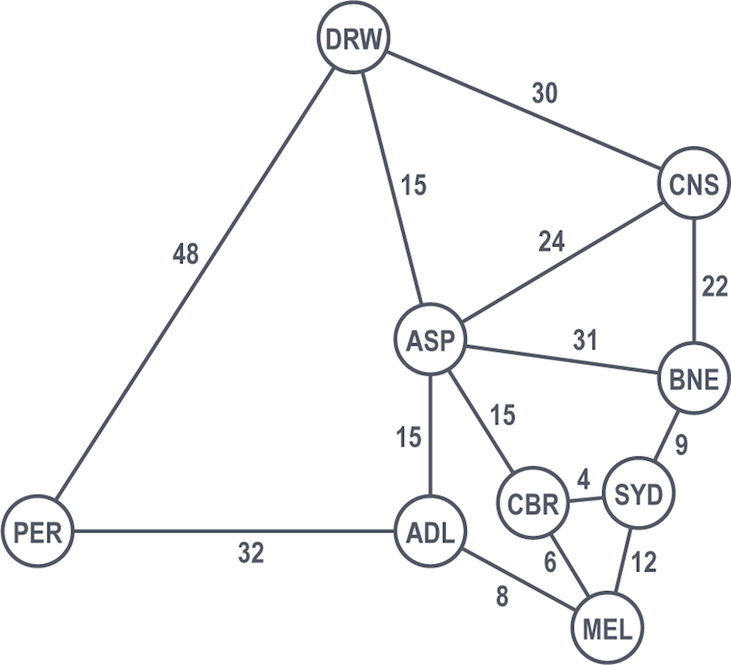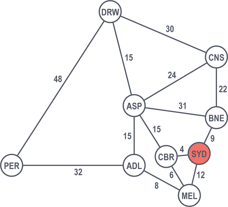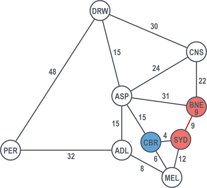Sydney is the start node and is immediately solved with a value of 0 as our famous duo are already there. Moving in a breadth-first manner, they look at the next cities one hop away from Sydney: Brisbane, Canberra and Melbourne. 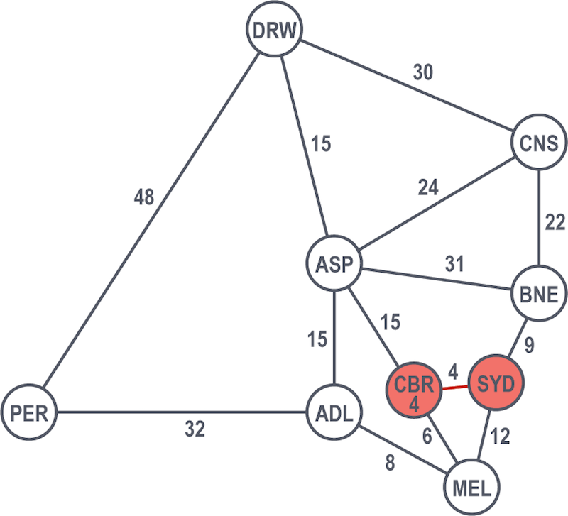Canberra is the shortest path at 4 hours, so they count that as solved. They continue looking at the rest of the graph from their solved nodes (from Sydney and from Canberra), considering other nodes and selecting the shortest path. From there, Brisbane at 9 hours is the next solved node. 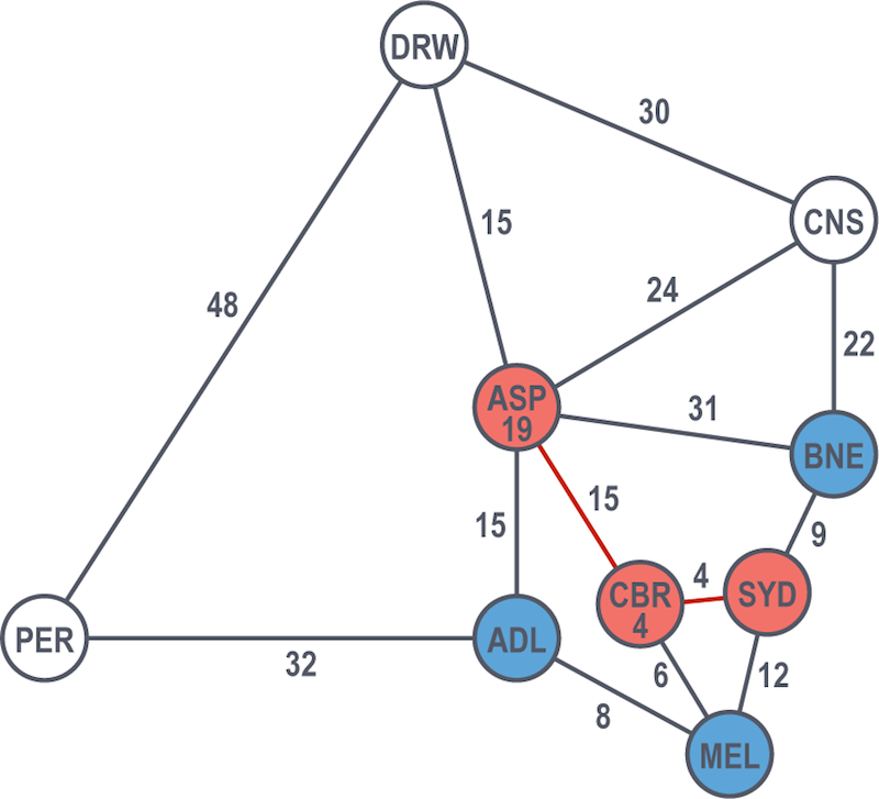They move on, choosing between Melbourne, Cairns and Alice Springs. Melbourne is the shortest (total) path at 10 hours from Sydney via Canberra, so it becomes their next solved node. Their next options of neighboring nodes (from already solved ones) are Adelaide, Cairns and Alice Springs. At 18 hours from Sydney via Canberra and Melbourne, Adelaide is the next shortest path. 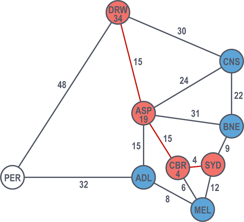The next options are Perth (their final destination), Alice Springs and Cairns. While in reality we know that they should next head directly to Perth, al-Khwarizmi and Euler are still sort of new to this whole “Australia even exists” concept. So, they decide to strictly follow Dijkstra’s algorithm no matter what (this is what a computer would do, after all). According to Dijkstra’s algorithm, Alice Springs is chosen because it has the current shortest path (19 total hours vs. 50 total hours). Note that because this is a breadth-first search, Dijkstra’s algorithm must first search all still-possible paths, not just the first solution that it happens across. This principle is why Perth isn’t immediately ruled out as the shortest path. From Alice Springs, their two options are Darwin and Cairns. The latter is 31 hours to the former’s 34 hours, so Cairns is the next solved node. The only unsolved node left from Cairns is Darwin. From Darwin, they make the final stretch and end up at Perth, with a cost of 82 hours for this given explored path. 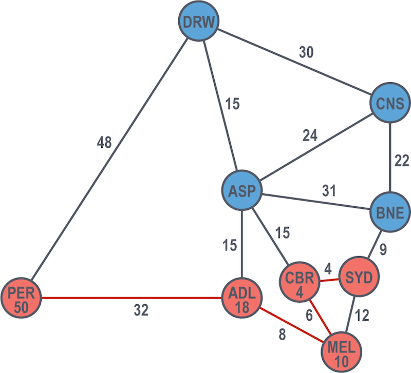Now that al-Khwarizmi and Euler have used Dijkstra’s algorithm to solve for all possible paths, they can rightly compare the two routes to Perth:

• • via Adelaide at a cost of 50 hours, or
  • via Darwin at a cost of 82 hours

Accordingly, Dijkstra’s algorithm would choose the route via Adelaide and consider Perth from Sydney solved at a shortest path of 50 hours. Let the road trip of the centuries begin. In the end, we see that the algorithm uses an undirected exploration to find its results. Occasionally, this causes us to explore more of the graph than is intuitively necessary, as Dijkstra’s algorithm looks at each node in relative isolation and may end up following paths that do not contribute to the overall shortest path. The example above could have been improved if the search had been guided by some heuristic like in a best-first search. To apply that in the road trip example, they could have chosen to prefer heading west over east and south over north, which would have helped avoid the unnecessary (mental) side trips.

The A* Algorithm

The A* algorithm improves upon Dijkstra’s algorithm by combining some of its elements with elements of a best-first search. Pronounced “A-star”, the A* is based on the observation that some searches are informed, which helps us make better choices over which paths to take through the graph. Like Dijkstra’s algorithm, A* can search a large area of a graph, but like a best-first search, A* uses a heuristic to guide its search. Additionally, while Dijkstra’s algorithm prefers to search nodes close to the current starting point, a best-first search prefers nodes closer to the destination. A* balances the two approaches to ensure that at each level, it chooses the node with the lowest overall cost of the traversal. As demonstrated by the example in the previous section, it is possible for Dijkstra’s algorithm to overlook a better route while trying to complete its search. For more information on how the A* algorithm is used in practice, consult Chapter 7 of Graph Databases from O’Reilly Media.

Conclusion

Graph search algorithms help you (or your friendly computer sidekick) traverse a graph dataset in the most efficient means possible. But “most efficient” depends on the results you’re looking for – a breadth-first search isn’t the most efficient if your results are better suited to depth-first queries (and vice versa). This is where your super-nerd friends (or even a helpful ebook, if you don’t have friends) come in handy. If they’re smart, they’ll match the right graph algorithm with the type of results you’re looking for. But now when they start talking breadth-first vs. depth-first vs. best-first you can tell them you know your A* from your Dijkstra and this isn’t your first rodeo. Go make al-Khwarizmi proud. Catch up with the rest of the Graph Databases for Beginners series:

• • Why Graph Technology Is the Future
  • Why Connected Data Matters
  • The Basics of Data Modeling
  • Data Modeling Pitfalls to Avoid
  • Why a Database Query Language Matters (More Than You Think)
  • Imperative vs. Declarative Query Languages: What’s the Difference?
  • Graph Theory & Predictive Modeling
  • Why We Need NoSQL Databases
  • ACID vs. BASE Explained
  • A Tour of Aggregate Stores
  • Other Graph Data Technologies
  • Native vs. Non-Native Graph Technology