Introducing GraphAware Databridge: Graph Data Import Made Simple

Principal Consultant, GraphAware
9 min read
GraphAware is a Gold sponsor of GraphConnect San Francisco. Meet their team on October 13-14th at the Hyatt Regency SF.
Introduction
Until now, Neo4j users wanting to import data into Neo4j have been faced with two choices: Create Cypher statements in conjunction with Cypher’s LOAD CSV or use Neo4j’s batch import tool.
Each of these approaches has its strengths and weaknesses. LOAD CSV is very flexible, but you need to learn Cypher, it struggles with large volumes of data and is relatively slow.
On the other hand, Neo4j’s batch import tool is extremely efficient at processing large data volumes. You don’t need to know any Cypher, but the input files usually need to be manually generated beforehand. Being a simple CSV loader, it also lacks the expressive power of Cypher.
Furthermore, many of the issues faced by any reasonably complex data import process can’t easily be solved using the existing tooling. Consequently, people often resort to creating bespoke solutions in code. We know, because we’ve done it enough times ourselves.
Databridge
At GraphAware, we didn’t want to keep re-inventing the wheel at every new client we went to. So we took a different approach and built Databridge. Databridge is a fully-featured ETL tool specifically built for Neo4j, and designed for usability, expressive power and impressive performance. It’s already in use at a number of GraphAware clients, and we think it’s now mature enough to bring it to the attention of the wider world.
So, in this blog post, we’re going to take a quick tour of the main features of Databridge, to give you an idea of what it can do, and to help you get a feel for whether it would be useful for you.
We’ll create a really simple example that you can follow along with as we go.
Declarative Approach
One of the difficulties with the current ETL tools is that they are quite developer-oriented. You either have to learn a lot of Cypher, or you have to be able to manipulate your raw data sources and generate node and relationship files that the batch import tool can use. As noted earlier, when these two options become infeasible, you need to write code.
But in fact, every Neo4j import needs to do exactly the same sorts of things: locate the data sources, know how to transform them into graph objects, link nodes together with relationships, assign labels, index properties and so on. All this pretty much boils down to two questions:
- What data do I want?
- What do I want it to look like when it’s loaded in the graph?
Databridge tackles these questions by being primarily declarative, instead of programmatic in nature.
It does this by using simple JSON files called schema descriptors in which you define the graph schema you want to build, along with resource descriptors in which you identify the data you want to import, and how to get it. This means you’re able to work directly with your source data exactly as is.
If you can create a JSON document, you can use Databridge.
Example: Satellites
In this example, we have some satellite data in a CSV file:
"Object","Orbit","Alt","Program","Manned","Launched","Status"
"Sputnik 1", "Elliptical","LEO","Soviet", "N", "04 Oct 1957", 0
"Mir", "Circular", "LEO", "Soviet", "Y", "19 Feb 1986", 0
"ISS", "Circular", "LEO","International", "Y", "20 Nov 1998", 1
"SkyLab", "Circular", "LEO", "NASA", "Y", "14 May 1973", 0
"Telstar 1" "Elliptical","MEO","International", "N", "10 Jul 1962", 0
"GPS USA66", "Circular", "MEO","International", "N", "26 Nov 1990", 1
"Vela 1A" "Circular", "HEO","NASA", "N", "17 Oct 1963", 0
"Landsat 8" "Circular", "LEO", "NASA", "N", "11 Feb 2013", 1
"Hubble" "Circular", "LEO", "International", "N", "08 Feb 1990", 1
"Herschel", "Lissajous", "L2", "ESA", "N", "14 May 2009", 0
"Planck", "Lissajous", "L2", "ESA", "N", "14 May 2009", 1
This data contains the following columns:
- Object: The satellite name
- Orbit: Orbital type (Elliptical, Circular or Lissajous)
- Alt: the orbital location (LEO=Low-Earth Orbit, MEO=Mid-Earth Orbit, etc.)
- Program: The space program that launched the satellite (NASA, ESA, etc.)
- Manned: A yes/no flag indicating whether the satellite was or is manned (e.g., Mir Space Station)
- Launched: The date the satellite was launched
- Active: A 1/0 flag indicating whether the satellite is still active
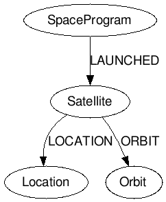
Of course, there are many ways you could choose to build a graph from this dataset, but for the purposes of this blog post, we’ll build a simple graph model like this:
Node types (Labels):
SatelliteOrbitLocationSpaceProgram
Relationships:
- A
Satelliteis related to anOrbitvia anORBITedge - A
Satelliteis related to aLocationvia aLOCATIONedge - A
SpaceProgramis related to aSatellitevia aLAUNCHEDedge
Schema Descriptors
Databridge lets you describe graph data models using schema descriptor files:
import/satellites/schema/satellites-schema.json
{
  "nodes": [
    {
      "type": "Satellite",
      "labels": [ { "name": "Satellite" } ],
      "properties": [
        { "name": "satellite", "column": "Object" },
        { "name": "manned", "column": "Manned" },
        { "name": "active", "column": "Status" },
        { "name": "launch_date", "column": "Launched" }
      ],
      "identity": [ "Object" ],
      "update_strategy": "unique"
    },
    {
      "type": "SpaceProgram",
      "labels": [ { "name": "SpaceProgram" } ],
      "properties": [ { "name": "program", "column": "Program" }],
      "identity": [ "Program" ],
      "update_strategy": "unique"
    },
    {
      "type": "Orbit",
      "labels": [ { "name": "Orbit" } ],
      "properties": [ { "name": "orbit", "column": "Orbit" } ],
      "identity": [ "Orbit" ],
      "update_strategy": "unique"
    },
    {
      "type": "Location",
      "labels": [ { "name": "Location" } ],
      "properties": [ { "name": "location", "column": "Alt" } ],
      "identity": [ "Alt" ],
      "update_strategy": "unique"
    }
  ],
  "edges": [
    { "name": "LAUNCHED", "source": "SpaceProgram", "target": "Satellite", "properties": [ { "name": "launch_date", "column": "Launched" }] },
    { "name": "LOCATION", "source": "Satellite", "target": "Location" },
    { "name": "ORBIT", "source": "Satellite", "target": "Orbit" }
  ]
}
As you can see, the nodes section creates a definition for each type of node we want in the graph. The columns from each row of data in the CSV file will be automatically mapped by Databridge to the properties of the node types we have defined.
In the edges section, we specify the three relationships we want in our graph data model. For each edge definition, we specify the name of the relationship, the start node type and the end node type, and optionally any properties.
Resource Descriptors
Now that we’ve defined the schema describing how we would like to map the CSV data to the various nodes, edges, labels and properties in the graph, we need to tell Databridge where to find the satellites data. This is the purpose of resource descriptors.
There are different resource descriptor formats for different resource types (a JDBC resource is not the same as CSV resource, for example). A CSV resource descriptor contains a resource attribute, and optionally an attribute describing the column names (for CSV data without a header row), as well as the delimiter. We will name our resource descriptor satellites-resource. This name will allow Databridge to automatically associate it with the satellites-schema file we created earlier.
import/satellites/resources/satellites-resource.json
{
  "resource" : "import/satellites/resources/satellites.csv",
  "delimiter": ","
}
Schema Control File
More often than not, an import will consist of many interlinking schemas and their associated resource definitions, so we need a way to bring them all together when we run the import. The schema control file (called schema.json) is where we do this. It’s a simple JSON file where we enumerate the schema definitions we want to include in the import, and the order we want to include them:
import/satellites/schema.json
{
  "include": [
    "satellites.json"
  ]
}
Running the Import
That’s it. Now, we can run the import. To do that, we’ll use Databridge’s command-line shell.
$ bin/databridge run satellites
This will run the import as a foreground task, so you will be able to observe its progress on the console. It should only take a second or so.
Databridge creates a completely new graph database, separate from any other that Neo4j is using, so you can’t corrupt or overwrite your existing graph database. If your Neo4j server is running on the same machine as Databridge, you can then use the shell to switch it to use the new database the import has just created:
$ bin/databridge use satellites
Switching to 'import/satellites/graph.db'
Password:
Starting Neo4j.
Started neo4j (pid 9614). By default, it is available at https://localhost:7474/
There may be a short delay until the server is ready.
See /usr/local/Cellar/neo4j/3.0.4/libexec/logs/neo4j.log for current status.
Graph database 'import/satellites/graph.db' has been deployed and Neo4j restarted
$
Finally, open the Neo4j Browser and explore your new graph!

Databridge Is Not Just for CSV
Although our example above used a CSV data source, Databridge is able to simultaneously consume different kinds of tabular data during an import:
- Text files
- CSV
- Note: Text-based resources can also be fetched over a network (using HTTPS, SFTP, SSH etc), so you don’t have to move your data files around if you don’t want to.
- Spreadsheets
- Microsoft Excel (2010 and later)
- Relational databases
- Oracle
- Microsoft SQL Server
- Teradata
- Sybase
- Informix
- IBM DB2
- Note: Databridge can also autoconfigure an import from any JDBC datasource by examining the database schema and automatically generating the appropriate Databridge schema and resource definitions for you.
Databridge Is Not Just for Tabular Data Either
Databridge also provides adapters for a number of non-tabular data resources with well-known formats. These include:
- Timetabling formats
- CIF (Association of Train Operating Companies)
- Navigation formats
- ITN (TomTom Itineraries)
- GPX (GPS Exchange Format)
- Vector geometry / geospatial formats
- WKT
If none of these fit the bill, you can easily build and deploy your own adapter, thanks to Databridge’s plugin architecture and simple Adapter API. Or ask us to help!
Filters
A fully-featured Expression Language lets you define which graph elements should be included or excluded while your data is being imported. You can define filters for nodes, labels, properties and relationships as well as supply default values for any missing properties.
Data Composition
You can compose data for a single node from different data sources. For example, you could create a common view of a Customer node in the graph by combining relevant information from a Sales database along with a CSV export from a Marketing database.
Strategies for Handling Duplicate Keys
CSV extracts and SQL queries that join tables often contain duplicate data. Databridge gives you total control over how you handle such duplicates by allowing you to specify update strategies for the different node types encountered during the import:
- unique (create the node only once, ignoring any duplicates)
- merge (create the node once, but update it if a duplicate occurs to merge in any additional properties)
- version (create a new version of this node each time – e.g., to maintain history of stock movements over time)
Data Converters
Databridge supports a wide variety of data converters, including:
Date Converters:
- unix_date
- long_date
- iso8601_date
- days
- julian
Number Converters:
- string
- floor
- ceil
- round
- real
- integer
And of course, if you can’t find the data converter you need, you can create a plugin to do it for you, using the Plugin API.
Other Features
Compatibility
Databridge works with all versions of Neo4j from 2.0 onwards.
Tuning
Databridge comes with a built-in profiler to help optimise huge data imports.
Shell
The Databridge command-line shell allows you to accomplish common import tasks easily and intuitively.
Performance
Databridge uses state-of-the art off-heap data structures to relieve JVM Garbage Collection pressure during the import. As a result, throughput scales linearly to hundreds of millions of nodes and edges, and it is quite easy to achieve import speeds of over 1 million graph objects per second on fairly ordinary hardware.
Supported platforms
Databridge works on all Debian-based and RPM/RHEL-based Linux systems, as well as Mac OS X.
There is currently no native support for Windows (we’re working on it!), but in the meantime, if you are on a Windows platform, you can install a guest VM of one of the supported platforms and run Databridge inside the VM, or you can install a Bash emulator like Cygwin or MingW32.
Conclusion
We firmly believe that Databridge represents a step change when it comes to data import for Neo4j. It’s been tried and tested in the field with a number of our own clients, and we’re confident it is suitable not just for SMEs but also for much larger enterprises.
We’ll be following up this introductory post with some in-depth tutorials very soon, where we’ll put Databridge through its paces, but in the meantime if you’re interested in Databridge, if you’d like a demo, or you want to discuss your data import problems with us, why not get in touch at info@graphaware.com?
We’ll also be at GraphConnect San Francisco so come on over and say hi!
Share Article


Explore
Related Articles


Integrating Neo4j With Symfony: Profiling Queries and Centralized Logging
Integrating Neo4j With LangChain4j for GraphRAG Vector Stores and Retrievers