(March Madness) <-[:MADE_SANE_WITH]- (Neo4j)

Neo4j Evangelist
4 min read

March GRAPHness
Download all the code needed to try it out for yourself HERE, or check out the GraphGist HERE.
March madness is a rare concord of well-documented data and pop culture. Warren Buffet’s billion-dollar bet grabbed the interest of everyone from Wall St. quants to Silicon Valley engineers to arm chair Money Ballers everywhere, and suddenly it paid off to be a big data geek.
It’s all relative
To me, basketball is all about relationships — there are of course teams that are unambiguously better than others. However, there nearly always some sort of relative performance bias.
Where a team performs better or worse than their average performance would project due to some confluence of factors, whether it’s a team with a infamously brutal crowd of fans, a Point Guard that dissects your league-leading zone, or a decades-long rivalry that motivates your players to dig just a little more.
Performance is relative. These statistics are difficult to track across a single season and often incredibly difficult to track across time.
Secondly, being able to iterate on that model is taxing both in terms of writing the queries and in maintaining any reasonable performance on commodity hardware. I had a mountain of data from the past four seasons, including points scored, location, date, etc. etc.
We could easily add more granular information or more historic data, but for no particular statistical reason and only because it made my life easier, I decided that in my model these relationships should churn almost entirely every four years (as current players graduate and move on).
Finally, we’re going to build our “win power” relationship between teams as a function of the Pythagorean Expectation model (More on that later).
STEP 1: Idea —> Graph model
I am not a clever boy. However, I have several clever tools at my disposal.
The most chief of which is Neo4j. So, I started as I do all of my graphy projects — with the questions I planned to ask most frequently and a whiteboard (or a piece of paper in this case).
Which became…

Which is a totally reasonable graph model for me to import data against.
STEP 2: Time
Before I loaded any data into Neo4j, I first needed to create the time-tree seen in the above model. One of Neo4j’s brilliant engineers (Thanks Mark!) did the heavy lifting for me and wrote a short Cypher snippet to generate the time-model I needed.

The result is something like this:

STEP 3: my.csv —> graph.db
Neo4j ships with a very powerful ETL tool called “LOAD CSV.” We’re going to use that.
I downloaded a mess of NCAA scores, then surreptitiously converted the data I downloaded from Excel spreadsheets into CSV format. I’ve hosted them in a public Dropbox found in the repo link above.
We’re bringing in several CSV files, each one representing a given season and then sewing that all together based on team names.

STEP 4: History, victory and a little math
I’ve decided to create a relationship between each team called :WINPOWER based on what’s called concept from baseball called Pythagorean Expectation.
:WINPOWER essentially assigns a win probability based on points scored vs. points allowed. I added in a decay factor to weigh more recent games more heavily than those played long ago.

STEP 5: The big payout
Who should win between Navy and Michigan St.?

We see that our algorithm predicts (correctly!) that Michigan St. will defeat Navy:

Well…but what if they’ve never played each other? We can use the other teams they both played in common to determine a winPower:

We see that Kentucky should (and did) beat Hampton!

// kvg
Want to learn more about graph databases? Click below to get your free copy of O’Reilly’s Graph Databases ebook and discover how to use graph technologies for your application today.
Share Article


Explore
Related Articles

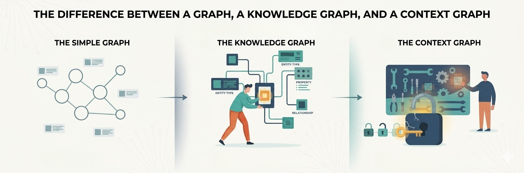
1 of 3: The difference between a graph, a knowledge graph, and a context graph
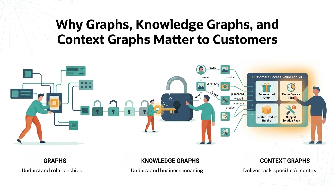
2 of 3: Why graphs, knowledge graphs, and context graphs matter to customers