
Editor’s Note: This presentation was given by Wren Chan and Sidharth Goyal at GraphConnect New York in October 2017.
Presentation summary
UBS set out to create a real-time data lineage tool in response to the new BCBS 239 regulations, which developed new risk-reporting requirements for financial institutions. This new data governance platform is called the Group Data Dictionary, which tracks data from its origins and how it moves over time, which is an important function to help ensure data integrity.
The UBS team originally built their governance platform in Oracle, but began the transition to Neo4j because data lineage, as a collection of highly connected data, is naturally more persistent in Neo4j. The data transfer process included APOC for a full sync, an incremental sync and a reconciler, a simple java app connection between the two databases.
Once the data was in Neo4j, the team developed four lineage generation algorithms. There are still several challenges with the lineage generation tool, including circularity, complexity, coupling and missing standards for graph formats. But the team is working on several enhancements related to graph transformation.
Full presentation: Real-time data lineage at UBS
What we’re talking about today is UBS’ Group Data Dictionary, an application to generate real-time data lineage:
Sidharth Goyal In the following presentation, we’re going to go over:
- Data lineage and data governance, which will provide an overview of our requirements, and how we implemented them.
- The Group Data Dictionary, which we built at UBS in the reference data space to capture metadata and generate data lineage.
- How we synced our data to Neo4j.
- Lineage generation, which is the meat of the data analysis we’re performing.
- Learnings, enhancements, and conclusions.
Data lineage and data governance
Data lineage allows us to track data origins and lifecycles, and analyze how data flows and changes impact an organization:

But why do we need data lineage?
Because it allows us to track data as it flows through an organization, which in turn is helpful for tracking errors, identifying data quality issues, and uncovering any of the impacts data changes may have on the organization.
The following example shows how data flows through four different applications:

If there’s an error in one of the attributes of a particular application, or a particular attribute is changed, you can easily see what other applications it will impact.
For example, if Attribute 2 in Application 3 is changed, this will impact Attributes 2 and 3 within Application 4. And while this is an extremely simplified use case, you can understand how important a tool like this is when you’re serving anywhere from 20 or 1,000 upstream users. Accurate data lineage will allow you to confidently know whether or not a change in an attribute is going to have a large impact on the flow of data.
We built our data lineage system in response to the Basel Committee on Banking Supervision’s standard number 239 (BCBS 239) regulation, which seeks to improve banks’ risk data aggregation capabilities and improve the bank’s reporting practices for overall data accuracy, integrity and completeness.
Building the Group Data Dictionary (GDD)
To perform all of these functions, we built a data governance platform called the Group Data Dictionary (GDD).
In simple terms, it’s an application that aggregates metadata about data for lineage generation. It performs the following functions:
- It takes into account all the assets we need to govern (applications, concepts, and entities).
- It manages our workflow. Users are able to input data, all of which goes through a four-eye check by Data Stewards and Owners to ensure data quality.
- These capabilities allow us to go back in time and audit our data to understand what changed when, who changed it, etc.
- Changes are reviewed and approved by Data Stewards and Data Owners, which helps ensure data is accurate.
Our tool also has generation capabilities. Once all the data is injected, we use
Neo4j to evaluate and compose the lineage into GraphJSON, which is then fed into a D3.js visualizer to render the data into a lineage diagram. And once we have all the accurate metadata in one location, we can export the lineage as an Excel file or do Ad Hoc reporting.
We built the first iteration of GDD and previously performed lineage generation in Oracle, but decided to shift to Neo4j. Data lineage is a series of highly connected data, and is more naturally persistent in a graph database. Cypher allowed us to much more easily traverse connected data, especially compared to PL/SQL, which relies on JOINS across multiple tables to generate the lineage in a relational database format, add a processing layer to format this as an object and then visualize it. Cypher and Neo4j are a much more natural fit for the work we’re trying to do.
GDD is also a data governance tool. There’s really no official model for data governance because every organization relies on a wide variety of data types and operates in different ways. But we do think the following model, which was developed by Collibra, came pretty close:

It builds the case that data governance can be divided into three categories:
- the asset model, which is the “what” of the data and lays out what needs to be governed
- the execution model, which talks about how the data is governed and its validation rules
- the stewardship model, which controls the “who” of data governance for quality control purposes.
The top of the asset model exists in a conceptual realm, while you move into the physical realm of data attributes as you move down the asset model:

An early iteration of the GDD was based on the bottom-up asset model, but our current version exists in the top half of the enterprise data model.
Within the reference data IT space, we’ve implemented a data distribution platform similar to GDD but that resides in the physical part of the asset model. We’re working towards being able to use the physical model to understand data as it flows from one consuming application to the other.
Now we’re going to walk through out metamodel, which we’ll tie back to the data governance model:
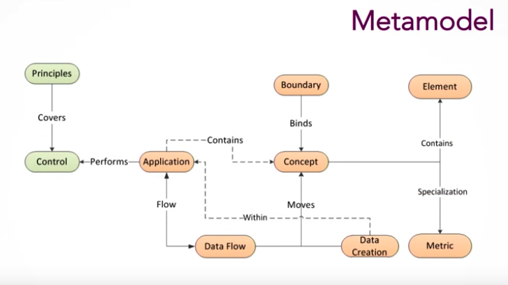
The assets, which are used to generate lineages, are represented in orange. The different types of assets include:
- Applications, which are the systems through which the data flows.
- Concepts, which are conceptual aggregations of physical data. A good example is a car, which is made up of steering wheel, tires, and an engine. All of these together form the concept of a car.
- Elements, which are the actual physical data.
This model allows us to ask questions like: How is all this data aggregated?
If we go back to our car example, we can find out where the car’s attributes come from, and how they flow through the entire organization and come together to form this one concept. These flows are configurable enough to show which application creates the data, which in turn allows you to see the direction and origin of data, which makes up the asset model.
The green in our chart represents principals and controls, which is essentially data monitoring. Apart from this, we have distinct rules for different types of users. Some users only have the permissions to edit data, while others must approve data and changes to data before they are accepted. This controls the “who” of data governance.
From Oracle to Neo4j in 3 steps
As I mentioned before, we started off using Oracle to generate our data lineages. Our main challenge was to move to Neo4j while keeping our workflows and audit capabilities. Additionally, at the time Neo4j didn’t have a proven concept of audit. This was the rationale behind deciding to synchronize Neo4j with our Oracle database.
Our real-time synchronization roadmap had three steps. We started with the full sync, which is an initial data load from Oracle into Neo4j. Next, we moved on to the real-time incremental sync, which propagated any changes that took place in Oracle into Neo4j. And finally, we created a reconciler to make sure that the databases were actually in sync.
Step 1: Full synchronization
In this stage, we started by creating procedures in APOC for each table in the Oracle relational data model, and then ran queries in sequence. We created all the assets, the chunk of data that’s governed by GDD. Then we created the data flows and linked all the assets together, which shows us how data flows between Neo4j applications. We also linked controls and applications to show how data quality is maintained:

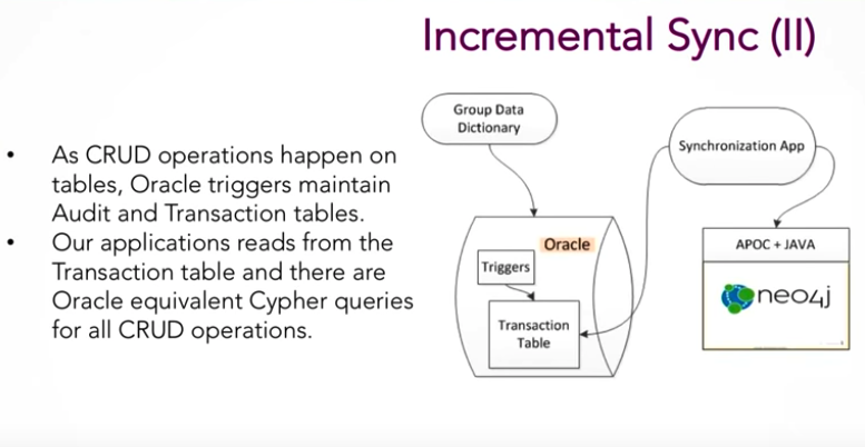
Step 2: Incremental sync
Next we looked into the incremental sync. We started on the Neo4j blog with the Monsanto use case. By using GoldenGate and Apache Kafka, Monsanto synced Oracle Exadata with Neo4j:

Because Monsanto had a high volume of data, they needed to add extra tools to their technology stack to make sure the sync worked. But because our use case has a low volume metadata repository, we kept our model pretty simple:
Using an Oracle table, we created a queue so that every time a user interacts with our application and makes changes to the database, triggers log these changes in a transaction table. Our synchronization application reads each of these transactions one at a time, and uses APOC and Java to persist those transactions into Neo4j.
Step 3: Reconciler
The reconciler is a simple Java app that connects to both Oracle and Neo4j, counts the number of assets in both databases, and makes sure both the counts and IDs match. This ensures that these databases are actually in sync.
Challenges
Even though our architecture is fairly simple, we did run into some challenges implementing it and ironing out all the wrinkles. Since all of our assets go through a workflow, they are frequently in different states.
For example, if the data has been approved by SMEs, they’re in a published state. If they haven’t been approved yet, they’re in a draft state:

To address this, we needed to provide users with a view of the latest data, regardless of whether or not it was still in draft (i.e. not yet approved by an SME) or published (i.e. approved by an SME). While the above example is the latest view of our data – because two attributes are still in draft – we can’t be confident that all the data is accurate. Therefore, for reporting purposes, we would only display assets that had been published.
Our second ingestion challenge was related to unpublished assets and rollbacks.
For example, if someone adds draft data incorrectly and links it to other data, you not only have to delete those assets because you have to delete its relationships too. This requried more maintenance than we wanted.
To deal with this, we created different namespaces. With each namespace, we run the same queries to generate the lineage, which simplifies the lineage generation part. Even though we now have to make changes in both namespaces, it only adds a little bit of complexity for us.
Lineage generation
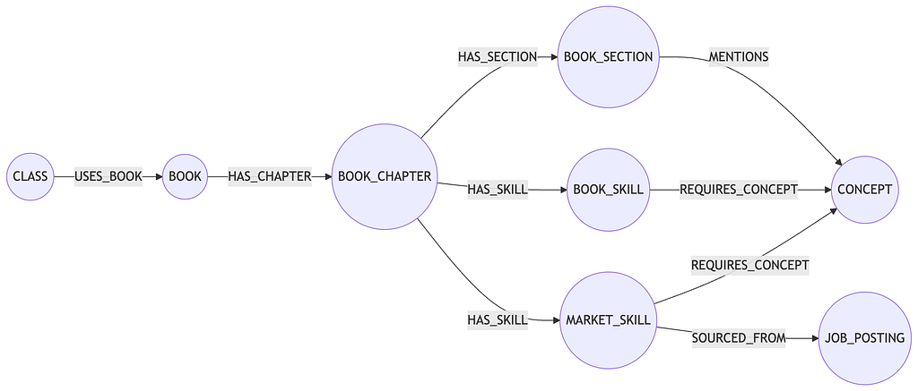
Wren Chan: Now let’s move onto lineage generation. As noted previously, lineage is used in the context of data governance to make sense of processed data. Below is an example of a lineage document that covers descent and title succession within the UK, which we’ll come back to later:

In this example, titles and houses are mapped to data concepts mentioned above. This gives a more concrete example of what a lineage diagram would look like.
We created four types of lineage generation algorithms:
- L1 is the initial algorithm that we developed through PL/SQL on an older data model, but with the performance optimized to 40 seconds. In the upcoming release, we plan to deprecate L1 in favor of L2.
- Our new L2 algorithm is effectively the same as L1, but is based on the new data model. Its current performance is for 30 seconds, but it hasn’t been optimized yet.
- L3 is a variant of L2 but with boundary intersections. A boundary is our way of designating how applicable a concept element is for a data flow. Think of it as we are putting an accumulator along a path, and using the results to determine whether or not to factor in an edge.
- L4 is a variant of L1 with a metric, which a special type of concept that Sid mentioned earlier. It ties back to the BCBS 239 regulation, because it’s a special report that tells us how the firm checks its risk. It’s currently implemented on top of L1, but we have the intention to migrate it over to Neo4j. Note that L4 is effectively a sub-graph of L1. So, in theory, we could actually use L1 as a pre-process step and just filter on top of that. We run another cipher query on top of L1.
This is how the L1 and L2 algorithm is broken down:

We initialize the filters and start the applications as mandatory and concepts as optional. We can drill down further to specify which specific concept to use as a filter in any given application. We traverse in both an upstream and downstream direction through the data flows that go in and out of that application.
Data creation can happen within an application when the application takes input data concepts and transforms them into something else. We iterate this through breadth-first on an additional linked application until there is no more edges found. At the very end, we compose all the paths that we find into a GraphJSON representation.
Below is the visualization of the L1/L2 lineage generation:

The yellow is our data distribution app. We go through the red concepts and paths on the first iteration. In our second iteration, we go through the risk calculation app, which calculates risk (blue) based on price and rating. It sends this to the reporting app, and the risk metric value is included in a report provided to regulators.
The boundary intersection for L3 is more complicated. It’s a condition set on applicability of the metadata for a concept. It’s broken down to the expression “key equals value.”
The example would be country equal UK, division equals ID, asset class equals equity. And then, you have expression sets which are composed with an operator, and the boundaries are composed of multiple expression sets. The evaluation boundaries intersection is effectively a cross-product of all the boundaries involved, which you can think of as Boolean algebra between all the expressions.
Like I said before, boundaries accumulate along a path, and if there are no intersections, the edge is not included.
Let’s go back to the UK title and lineage example from before:
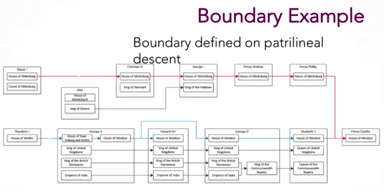
If you start with Queen Elizabeth and trace only the patrilineal descent back the earliest recorded founder of her line (shown in blue), Prince Charles wouldn’t be in that line because gender is the boundary condition. If you use Prince Charles as a starting application (red line).
Below is an example of an intersection:

The boundaries get more restrictive as you do across products, so eventually there is a point where a path is no longer viable.
Below is an example of when a path is no longer viable:

There are no further intersections, so we don’t proceed down the associated path. As noted, boundaries intersections are applied additively, so the boundaries will become more restrictive with each hop.
Lineage challenges
We have encountered several challenges related to lineage generation with Neo4j:
- Circularity. We have to avoid walking over an edge twice. The fault behavior is RELATIONSHIP_GLOBAL, which is when a relationship cannot be traversed more than once, but nodes can. We opted for a RELATIONSHIP_PATH, which says that for each returned node there’s a relationship wise unique path from the start node to that node. Unfortunately this will impact our performance, but we’ll perform some optimization, like memorization, to make it work.
- Complexity. We chose Neo4j so that BAs could translate to business requirements efficiently to maintain algorithms. But the current implementation relies heavily on APOC and Java, so while it helps make unit testing easier, it makes it less readable and maintainable. We’re working on improving this with the help of Neo4j.
- Coupling. With our current data model, there is a lot of coupling. We coupled the current data model in Neo4j with both Oracle and the presentation layer, which is effectively another graph. We have to massage the data in order to make our algorithm work.
- Missing Standards for Graph Formats. JSON formats include GraphJSON introduced by Alchemy.js to visualize graphs, but there are other JSON formats that are similar in structure. Neo4j provides an output that switches the edges to relationships if you pass an option in your Cypher query
( {resultDataContents":["graph"]} ).There are also XML equivalents of these formats that existed before JSON, including GraphML, DGML, GXL and XGMML. GraphML is one of the more popular ones that is supported by Neo4j as an output.
Enhancements
We’re working on several enhancements, including one to reduce coupling with the presentation layer.
This could be achieved by relying on graph transformation to create the final data lineage diagram, but this adds a layer of complexity because graph transformation is a complicated problem. There was a graph transformation conference earlier this year that bore two potential solutions.
The first is Graph Rewriting and Persistence Engine (GRAPE), which is an enclosure that you can actually run on top of Neo4j to do graph transformation. We’re also considering leveraging an APOC procedure that creates virtual Nodes/Rels/Graph. This may be closer to what we want, but again, we have to write out the logic of what our transformation entails.
There’s also the possibility that we could rely on the functionality of the newest Neo4j version to enhance our diagrams.
Conclusion
We’ve come across a number of lessons learned throughout this process. Moving from the relational to graph point of view was very hard for us. We’re so used to relational databases that it’s tough for our developers and BAs to understand the functionalities and limitations of graph databases. And since we have to audit everything within UBS, a relational database makes more sense for us.
Translating the user requirements is also challenging because in order to do graph properly, you need to apply the appropriate constraints on it. Most of the graph algorithms have an empty complete nature. If you remove the constraints, it means that your algorithms can’t complete in polynomial time.
One of the difficulties is finding a tool to ensure that we have enough coverage for all the test case. There are already Java and cold coverage plugins that tell us the number of lines and branches that have already been covered, but we don’t have that with Neo4j. GDD is still very much a work in progress.
Share Article


Explore
Related Articles

Hey LLM, you’re using OPTIONAL MATCH wrong. Here’s the Cypher that actually works.