Sentiment and Social Network Analysis

Editor’s Note: This presentation was given by Laura Drummer at GraphConnect New York in November 2017.

Presentation Summary

Traditional social network analysis is performed on a series of nodes and edges, generally gleaned from metadata about interactions between several actors – without actually mining the content of those interactions.

By pairing this metadata with data and communications content, Novetta’s SocialBee can take advantage of this widely untapped data source to not only perform more in-depth social network analysis based on actor behavior, but also to enrich the social network analysis with topic modelling, sentiment analysis and trending over time.

Through extraction and analysis of topic-enriched links, SocialBee has also been able to successfully predict hidden relationships that exist in an external dataset via different means of communication. The clustering of communities based on behavior over time can be done by looking purely at metadata, but SocialBee also analyzes the content of communications which allows for a richer analysis of the tone, topic, and sentiment of each interaction.

Traditional topic modelling is usually done using natural language processing to build clusters of similar words and phrases. By incorporating these topics into a communications network stored in Neo4j, we are able to ask much more meaningful questions about the nature of individuals, relationships and entire communities. Using its topic modelling features, SocialBee can identify behavior-based communities within this networks.

These communities are based on relationships where a significant percentage of the communications are about a specific topic. In these smaller networks, it is much easier to identify influential nodes for a specific topic, and find disconnected nodes in a community.

This talk explores the schema designed to store this data in Neo4j, which is loosely based on the concept of the ‘Author-Recipient-Topic’ model as well as several advanced queries exploring the nature of relationships, characterizing sub-graphs, and exploring the words that make up the topics themselves.

We’ll walk through the basics of a social network analysis using a test dataset, the fundamentals of topic modeling and a demo of how it all works in Neo4j.

Full Presentation: Sentiment and Social Network Analysis

What we’re going to be talking about today is how SocialBee uses Neo4j to conduct sentiment and social network analysis:



My name is Laura Drummer, and I work for a company called Novetta. We work primarily in the area of government consulting, and have a few software offerings in the realm of entity analytics, cyber analytics and something we call media analytics, which is a lot of Twitter and news parsing.

Before coming to Novetta, I worked as a Chinese Linguist and then a cyber analyst at the Department of Defense. I started as a data scientist and then a cyber analyst at Novetta, and now serve as the Director of Software and Engineering.

We’re going to start by going over the problem we’ve been trying to solve, which is that traditional social network analysis doesn’t include an analysis of the communications content; an exploration of the fundamentals of social network analysis; the fundamentals of topic modelling; how we bring it all together in Neo4j; and finally we’ll walk through a demo of analytic queries using Cypher.

What Problem Are We Trying to Solve?

Our challenge is that a traditional social network analysis often only looks at relationships between actors, and not what they’re actually talking about. This means that, while we might know that two people have a relationship, we don’t know what’s actually going on within that relationship.

Traditional social media analysis (SNA) ignores the two right columns in the following table:



Based on the information in this table, when we look through our organization’s emails, we find weekly emails from both the IT department and the CEO.

Based on the shared information under frequency and directionality for these two email types, you might to think relationships are similar – but, you’re probably going to take a little more time to read the CEO’s emails than those from the IT department (or vice versa).

And if I’m trying to target a bad actor’s organization, I’m likely going to care more about one email type than the other.

With my prototype, which we call SocialBee, we try to solve this problem:



The left is traditional network analysis, and the right is SocialBee’s analysis. We use topic modeling to turn the unstructured communications data into structured data, and then enrich the relationships with that information.

In this example, Alice emails Bob about work and social things, Bob emails Cara about work but also fraud, but Bob never emails to Alice. I don’t know what this tells me – but I know this tells me something, and it makes Bob’s relationships more interesting to me.

A helpful side effect of this technique is that we can predict relationships based on behavior similarities:



Even though you can do that with traditional social network analysis – for example, these two people aren’t friends but they have friends in common, so they may know each other – we take it a step further.

We can actually see that they spoke about the same things or behaved in similar ways based on analysis of the unstructured text associated with their relationship. We now know that not only is this person a friend of a friend, they are also a friend of a friend that talks about the same thing.

Sometimes we’ll find that these two people are actually the same person, which is a problem Novetta explores a lot called entity resolution. When this works, you can identify hidden relationships that can also help with entity resolution.

The Fundamentals of Social Network Analysis

Now let’s dive into the basics of social network analysis:



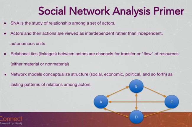
We’re really looking at the way people behave within a community of actors. Instead of just seeing that one person sends 60 emails a week, you’re looking at the directionality of who they email, and how their behavior compares to that of others within their community.

While in this case we’re analyzing people within a network who are interrelated, you can use this same technique for anything, including computers, to uncover the nature of relationships.

An easy way to map a network is to create a matrix:



We can use a 1 to indicate the two people know each other, and a 0 if they don’t. If we want to track how often they communicate, we can put in a number greater than 1 to indicate how frequently they communicate. The point is, these are all numbers, which is important because we’re going to use math to manipulate these numbers and turn out helpful data.

There are 15 people in this organization, represented by the 15 nodes, and the 25 edges indicate the number of relationships between these people. We can also calculate the network density, which describes the portion of the potential relationships in a network that are actual relationships. This is calculated by dividing the number of actual connections by the number of potential connections.

In this case the network density is .24, showing that it’s not a very interconnected network. The degree refers to the number of neighbors each person has, which is a minimum of two and a maximum of six. The average is a little over three.

This data is a lot more helpful if you can visualize it, like we did below:



There are a variety of indicators in this network that point to importance: the size of the node, which changes based on the number of degrees; and the shading, which refers to the centrality (i.e. how many people have to go through you to get to somebody else).

In this example, Emily has four friends, which is a fair amount compared to the network average of 3.3. But, if you don’t know anyone on that right side of the network, you have to go through Emily, which makes her even more important.

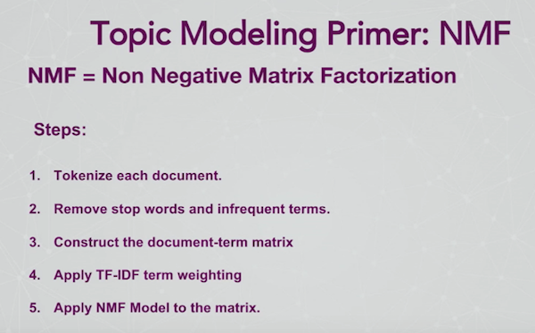
Topic Modeling Fundamentals

I use an algorithm called NMF, which stands for non-negative matrix factorization. A non-negative matrix is a matrix where every value is zero or greater, so there are no negative numbers. Then we factor the matrix, which has the nice side effect of clustering attributes together:



Let’s look at the following example of a document term matrix:



To construct this matrix, we created columns across the top for each word we found in a collection of documents, and along the left side we added a column for each document within the corpus, which in this case was made up of emails. We then added a value that corresponded to whether or not a particular word was contained in a particular document.

This is a sparse matrix because most words are not in most documents, resulting in a lot of zeros. This helps visualize what the algorithm is doing behind the scenes, and it’s easy to start doing some topic modeling with our eyes.

We can already see that the words bank, money and finance are used together a lot in Document 2. In a matrix, these colors would be numbers, with the darker color corresponding to more mentions. Document 1 has the words sports, club, and football, so is probably about something like Monday Night Football.

This represents a really really high-level version of what I’m doing with NMF, except I also include structured text to create a social network map. I’m going to apply this non-negative matrix factorization to the content of what they are sending to each other.

We also have a concept called the Author-Recipients-Topic Model (or the ART model):



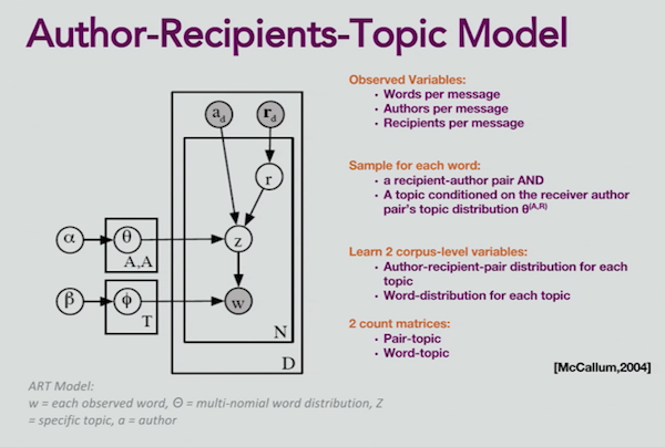
Now we’re not only grouping words, but we’re saying who is sending these topics to who. This comes from an article published by Andrew McCallum in 2004 about LDA, which is a Bayesian topic modeler.

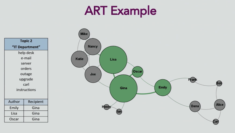
For this example, I’ve produced five different topics: the operations of my company, the IT department, annual performance reviews, the holiday party, and emails related to employees’ families:



If you’ve worked with topic modeling, you know that the results are usually much messier than this, but I wanted to provide some simplified data so that we can more easily walk through what we created with Neo4j.

What’s special with this type of topic modeling is that we also include the author and the recipient. Joe is the top sender of operations information, which he sends to Lisa. A lot of people email Gina about the IT department, so she probably works on that team. Nancy is emailing a lot of people about the annual review, so she might be a boss soliciting information about employees.

Our Neo4j algorithms measure trends over time. At the start of the assessment period, Nancy is sending a number of emails, but as everyone is turning in their assessments, now they’re all emailing Nancy. But at this point in time, she’s the top author, and Katie, Lisa, and Mike are the top recipients. For topics 4 and 5, the communications are pretty bi-directional.

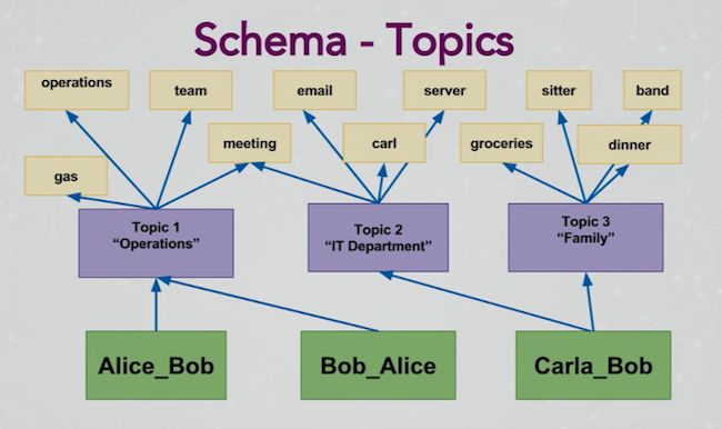
The idea behind this is to store this ART model in Neo4j, which allows us to start identifying sub-networks within our graph:



Again, this is based on what people are talking about, not on who is connected to who. I drew the lines using normal social network analysis, and now we’re highlighting certain areas of the map based on what topic they’re talking about. The above map shows the subgraph of people who are talking about operations.

This is really helpful in the areas of intelligence and law enforcement. For example, maybe somebody is following ISIS on Twitter, but somebody else is tweeting about how to make IEDs. We need both of those pieces of data, which we then put all together in Neo4j.

Here’s a social graph of the IT department conversations, with Gina managing the bulk of the emails:



And here’s a map of the annual review topic, with poor Lisa talking to everyone:



The graph for the familial topic is a bit more interesting:



Maybe these people have a friendship outside of work, or maybe they’re in a family. There’s no link between these two groups, and they’re probably not talking about each other’s families to each other. But if we consider ISIS cells, let’s say these people are talking about building bombs.

The two groups might actually be talking to each other somewhere separate from where our data is, which is where those hidden relationships comes into play. In fact, we may be missing data. And because we don’t always have the full picture, we have to make inferences from what we know to draw new links between communities.

We ran our prototype on the Enron email corpus, and we ended up with really interesting results. Most of you are probably familiar with the Enron scandal from 2001, in which a bunch of emails were released to the public because of a Freedom of Information Act request. It’s a great source of unstructured data that can be linked:



We take the raw text from the header in a general email, parse out the header, and send it to traditional network analysis with NetworkX and Python. Then we send the message content to our NMF topic modeler, which is where Neo4j is really powerful.

Below is the overall schema I designed for this data:



Some might question why I didn’t make the words or topics attributes. And that’s always where the fun comes in when you’re building a new Neo4j schema: what’s an attribute and what’s a node?

The idea behind this schema is that we want all of these to be seeds, or starting points for when we sit down with our big hunk of data. Do I want to start with a person and see who they talk to? Or do I want to start with a topic and see what the resulting network looks like? Or maybe I just want to start with exploring a single word.

Let’s zoom in on our schema:



We still maintain our directionality, and you can see that Alice and Bob know each other. The “know” relationship is actually one that exists in Neo4j, and provides the ability to do some really basic queries. But we also start storing information about their relationship, with all of their messages feeding into the big green nodes. This might contain information like “Alice emails Bob six times a day, but he only writes back once.” What does that tell us about their relationship?

This is where you can start exploring how words interact across topics:



If you were to run this model on all of the communications of 10 Enron executives, this is what the network would look like:



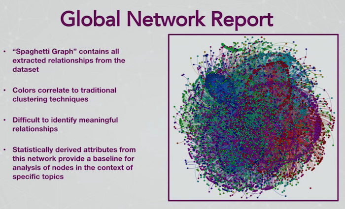
It’s completely pointless. I wanted to include a real data “hairball” to demonstrate some data challenges that we frequently run into, but I’m also going to show you how our algorithm takes this hairball and turns it into something useful.

What if I want to look at just one topic? Below is a graph of data from the Enron dataset about fantasy football:



These five main nodes represent five people who are quite influential. There are a few isolated networks off to the side, which represent people who are probably in a different league. This is simply the same dataset as the hairball above, but the data filtered down through Neo4j by the subject of people are actually talking about: fantasy football.

We’re also able to uncover some hidden relationships:



We have these two different people highlighted, and our algorithm thinks they know each other based on the frequency and content of their communications. To test our algorithm, we hid about a third of the Enron data to develop some predictions. We compared our predictions with the actual data and found that most of the time, our algorithm was quite accurate.

Social Network Analysis Demo