Super (Data) Model: Graphing “RuPaul’s Drag Race”

Senior Pre-Sales Consultant, Neo4j
6 min read

It’s that time of year, y’all… “RuPaul’s Drag Race” is back! At least in the UK… and, at least, that’s what I’ve been told.
I’m a newcomer to the “Drag Race” party, you see. I’ve always liked RuPaul but, in general, I avoid reality television programming and never managed to get into past seasons of “Drag Race.” This year is different though – I have some new folks in my social circle and they seem to talk about “Drag Race” all the time. My rapid descent into “Drag Race” fandom was unavoidable.
Rather than “dragging” my heels and moaning about it, I’ve decided to use this as a teachable moment. These new friends of mine have no idea what a graph database is, and so it’s very hard to convince them that I spend my weekdays actually working instead of watching old teen films and walking my dog.
What better way to explain Neo4j than to graph “Drag Race” for them! I’m up to the task – I have the Charisma, Uniqueness, Nerve and Talent to make the best “Drag Race Graph” you done ever seen.
Ready? ‘Cause if you want to understand graph databases, you better work!

To get started, I searched around the internet for data about the show and found a recent data science effort called RuPaul-Predict-a-Looza, which tries to build analytical models to predict the winners and losers of upcoming “Drag Race” episodes before they air.
I was relieved to find that I wasn’t the only data geek to be looking at the show in this way! Their dataset was exactly what I was looking for, so I loaded it into Neo4j.
Here’s the data model I came up with:
CALL db.schema()

The structure of the graph really focuses on two primary types of nodes: Contestants and Episodes.
We have some information about where Contestants come from – their Home Towns and their Home States.
We can see which Season each Contestant appeared in, as well as their season Ranking (with a ranking of ‘1’ being the season’s winner). Each Season has a number of Episodes, and each Episode has a Type (Casting, Competition, Finale, Recap or Reunion).
Each Competition Episode also has a Maxi-Challenge Type (Comedy, Personal Branding, Acting, etc.), which tracks what kind of main challenge the Contestants had to face in that Episode.
Between Contestants and Episodes, we have a number of relationship types that describe the outcome for each Contestant in the Episodes in which they appeared. We can see who Won an Episode, who was in the bottom two but not eliminated, who was eliminated, etc.
Now that we understand how our graph is structured, we can have a look at the data and explore the graph in more detail. For instance, I have it on good authority that Season 4 is really “Drag Race” at its best.
An overview graph for this season looks like this:
MATCH (c:Contestant)-[ais:APPEARS_IN_SEASON]->(s:Season {number: 4})-[he:HAS_EPISODE]->(e:Episode)
MATCH (c)-[hsr:HAS_SEASON_RANKING]->(r:Ranking)
MATCH (e)-[ht:HAS_TYPE]->(et:EpisodeType)
OPTIONAL MATCH (e)-[hmct:HAS_MAXI_CHALLENGE_TYPE]->(mct:MaxiChallengeType)
RETURN *

We can see that there were 11 Competition Episodes in this Season, along with a Recap Episode, a Finale Episode and a Reunion Episode.
There were three Episodes with an Acting challenge and two with a Sewing challenge, while the rest of the Episodes in this season had distinct types of challenges: Singing, Personal Branding, Makeover, etc.
There were 13 contestants in this season; and since Alissa Summers was eliminated first, she has a Ranking of 13. There were two runners up in Season 4, each with a Ranking of 2 – Phi Phi O’Hara and Chad Michaels. The winner of Season 4 was Sharon Needles, and if we look at her graph in more detail we see the following structure:
MATCH (hc:City)<-[ht:HOMETOWN]-(c:Contestant {name: 'Sharon Needles'})-[r]->(e:Episode)<-[he:HAS_EPISODE]-(s:Season)
MATCH (c)-[hs:HOME_STATE]->(st:State)<-[i:IN]-(hc)
OPTIONAL MATCH (e)-[hmct:HAS_MAXI_CHALLENGE_TYPE]->(mct:MaxiChallengeType)
RETURN *


Sharon hails from Pittsburgh, Pennsylvania and according to her she looks spooky but is really nice. Before being announced as the winner of Season 4: Episode 14, she won four episodes – with a Sewing challenge, a Commercial challenge, an Acting challenge and a Ball challenge. Her strength seems to be Acting challenges, since she won one and was in the High Group (up for consideration as the winner) for another. She seems to have had a more difficult time with her Makeover challenge (she was in the Low Group, for consideration in the bottom two) and her Singing challenge (she was in the bottom two and had to lip sync for her life).
I’m curious how contestants from my Home State have fared.
I was born in Connecticut, but I lived in New York for so long that I consider it home. I’m proud to say that New York has produced the most “Drag Race” Contestants of any state (28 in total, 25 from New York City) including three winners! You go, New York!
MATCH (r:Ranking)<-[hsr:HAS_SEASON_RANKING]-(c:Contestant)-[h:HOMETOWN]->(ht:City)-[:IN]->(:State {name: 'New York'})
RETURN *

In the spirit of the RuPaul-Predict-a-Looza, I’m also curious to see what kinds of insights we can get from our graph.
One common graph use case in industries like retail, telecom and other B2C and B2B business models is Customer Journey Analytics – looking at a series of events or actions by a customer and seeing if there’s a pattern we can use to predict outcomes.
For example, it might be that there are patterns of events in a customer’s history – purchases, complaints, account changes, social media posts, etc. – which indicate that they are about to “churn” or take their business elsewhere.
I wonder if there’s a pattern of contestant results that’s common to winners of each “Drag Race” season.
Let’s look at the results from the first three challenges each season winner faced, and see if there are any commonalities:
MATCH (:Ranking {position: 1})<-[:HAS_SEASON_RANKING]-(c:Contestant)-[result]->(e:Episode)
WITH c, result, e order by e.number
WITH c, collect(type(result)) as resultTypes
WITH c, collect([resultTypes[0], resultTypes[1], resultTypes[2]]) as firstThree
RETURN firstThree, count(c) as frequency, collect(c.name) as contestants
ORDER BY frequency DESC

Of the 11 season winners, we can see seven of them each had their own unique patterns of results in the first three episodes of their seasons. Two of them – BeBe Zahara Benet from Season 1 and Bob the Drag Queen from Season 8 – were both Safe in Episode 1, were both Safe in Episode 2, and both Won Episode 3 of their respective seasons.
We can also see that another two winners – Bianca Del Rio from Season 6 and Violet Chachki from Season 7 – both Won Episode 1, were in the High Group in Episode 2, and were Safe in Episode 3 of their respective seasons. While not hugely significant from a statistical standpoint, these shared patterns of winners’ results are certainly interesting.
If we look for this pattern in the Contestants of “Drag Race” UK Series 1, hoping to predict the winner, we might put our money on Divina De Campo. She fits the first pattern above and was Safe in Episode 1, Safe in Episode 2 and Won episode 3 (with a fierce Bowie-esque look made from plaid plastic carrier bags).
You heard it here first!

Now it’s time for me to sashay away, though I’ll be back to graph another day.
If you followed along with today’s blog post and have even more ideas about how to use our Drag Race Graph, then condragulations – you’re officially a Graphista! If not, then I’m sorry, dear, but you’re up for elimination (just kidding, sort of).
Either way, remember: If you can’t love yourself, how the hell are you going to love somebody else? Can I get an amen?
[Graphs are everywhere – even on the runway! This is another example of a knowledge graph, and there are so many ways we could further expand and enrich it – with social media data, for example, or information about how the contestants got along with each other (or didn’t) during the season. Knowledge graphs can be used to represent any information domain, from tea to “Drag Race” to engineering data from NASA. The sky’s the limit!]
Share Article


Explore
Related Articles


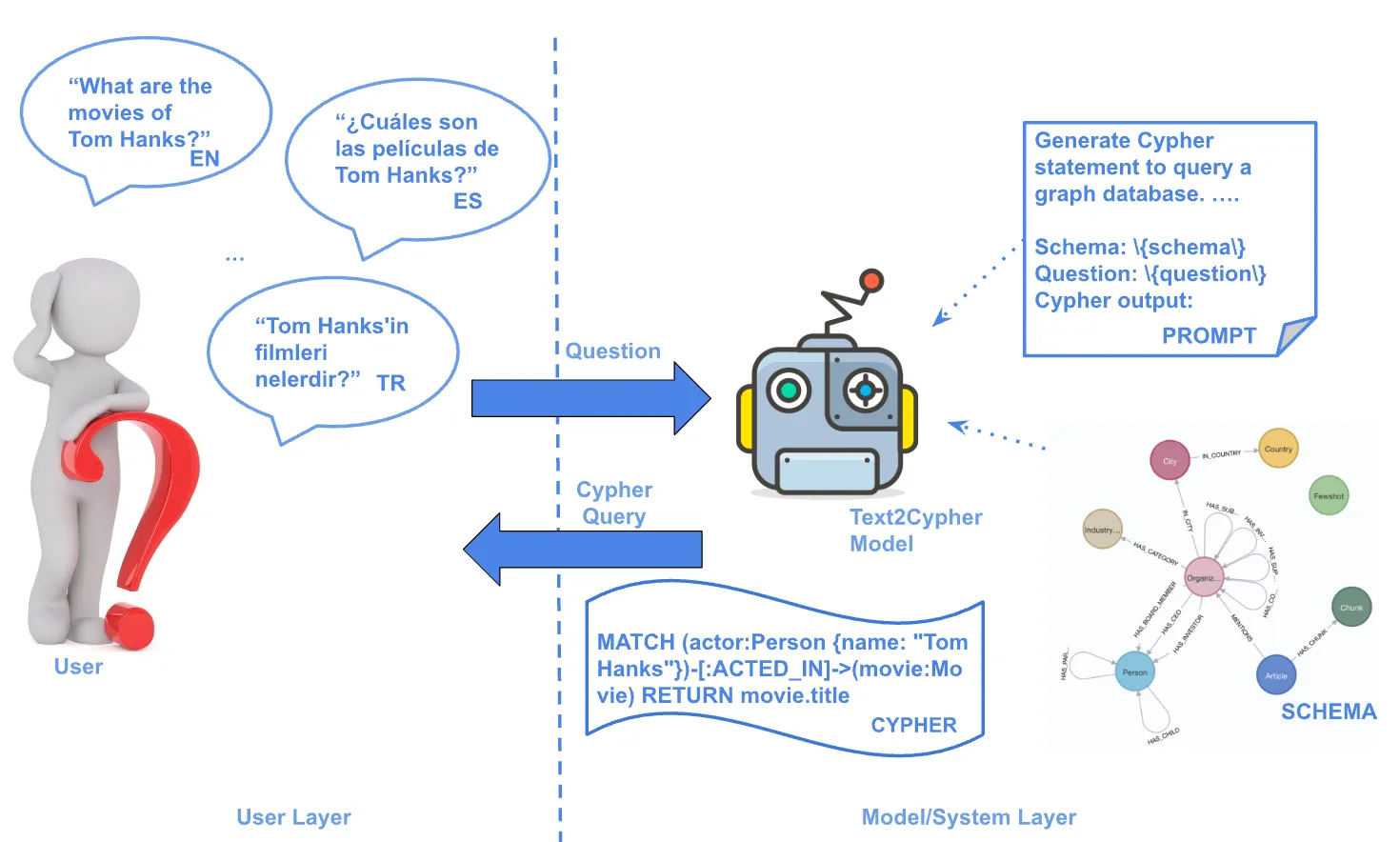
Text2Cypher Across Languages: Evaluating Foundational Models Beyond English