How to use phone calls and graphs to identify criminals?
11 min read

Originally posted on the Linkurious Blog
Call records are a great source of information on real life networks. We are going to see how graph technologies can be used to analyse these records in order to find potential criminals. That article has been written with the assistance of Ashley Englefield, Detective in California and instructor at Police Technical.
How to use phone calls to identify criminals?
The fact that a mobile phone can be a dangerous thing to have for a professional criminal has entered the popular culture a while ago. In the Wire for example, drug dealers use “burners”, cheap phones they dispose of regularly. Why? because your phone operator is authorized to collect information about whom you call, for how long and from where. In certain circumstances, that data can be used by law enforcement. But do you know the techniques used by police officers to use phone data to aid in arrests and convictions?
We are going to see how using graph technologies it is possible to analyse phone calls to find criminals.
To illustrate our use case, let’s use a common scenario. In a residential neighborhood, a store robbery is committed during the day by a group of 4 criminals. The criminals are masked, use a stolen vehicle and leave no fingerprints. In that kind of case, finding an answer may take a lot of legwork. A witness noticed that one of the criminal used his phone to make a call minutes before the crime.
Equipped with a search warrant, a police officer can contact mobile phone operators to collect information about the calls made and received near the robbery when it happened.
Data model to analyse the network in the phone calls
The data phone operators provide law enforcement is highly tabular. Trying to identify unique phone numbers and their relationships in tabular data is very hard. We are thus going to use the phone calls data to build a graph. That graph will show how the phone numbers are connected by phone calls. From a list of calls, we are inferring a network.

Finding relationships within a spreadsheet is hard.
For this article, we have prepared a small dataset using Mockaroo. That data is in a spreadsheet format. Here are the columns :
- FULL_NAME : full name of phone subscriber ;
- FIRST_NAME : first name of phone subscriber ;
- LAST_NAME : last name of phone subscriber ;
- CALLING_NBR : phone number of the caller ;
- CALLED_NBR : phone number of the person called ;
- START_DATE : start of phone call ;
- END_DATE : end of phone call ;
- DURATION : duration of phone call ;
- CELL_SITE: ID of cell site used to route phone call ;
- CITY : city of cell site used to route phone call ;
- STATE : state of cell site used to route phone call ;
- ADDRESS : address of cell site used to route phone call ;
We are going to use the data stored in the spreadsheet to build a graph. In order to do that, we need to define a graph model.

Graph model to represent the phone calls.
You can see above that our graph model for phone calls is centered around calls. A single phone call connects together 4 entities : 2 phone owners, a location (the cell site the caller was next to when he initiated the call), a state and a city.
It is important to note that in real life, most of the time we would not have access to the names of the phone numbers owners.
Importing the call records
Now that we have defined a model, we are going to populate it with the data stored in the spreadsheet. To store our graph, we will use Neo4j, a popular graph database. Neo4j has a language called Cypher that makes it easy to import csv files.
Here is a script that can turn our data into a Neo4j graph :
|
//Setup initial constraints
CREATE CONSTRAINT ON (a:PERSON) assert a.number is unique;
CREATE CONSTRAINT ON (b:CALL) assert b.id is unique;
CREATE CONSTRAINT ON (c:LOCATION) assert c.cell_tower is unique;
CREATE CONSTRAINT ON (d:STATE) assert d.name is unique;
CREATE CONSTRAINT ON (e:CITY) assert e.name is unique;
//Create the appropriate nodes
USING PERIODIC COMMIT 1000
LOAD CSV WITH HEADERS FROM “file:c:/Users/Jean/Downloads/call_records_dummy.csv” AS line
MERGE (a:PERSON {number: line.CALLING_NBR})
ON CREATE SET a.first_name = line.FIRST_NAME, a.last_name = line.LAST_NAME, a.full_name = line.FULL_NAME
ON MATCH SET a.first_name = line.FIRST_NAME, a.last_name = line.LAST_NAME, a.full_name = line.FULL_NAME
MERGE (b:PERSON {number: line.CALLED_NBR})
MERGE (c:CALL {id: line.ID})
ON CREATE SET c.start = toInt(line.START_DATE), c.end= toInt(line.END_DATE), c.duration = line.DURATION
MERGE (d:LOCATION {cell_tower: line.CELL_TOWER})
ON CREATE SET d.address= line.ADDRESS, d.state = line.STATE, d.city = line.CITY
MERGE (e:CITY {name: line.CITY})
MERGE (f:STATE {name: line.STATE})
//Setup proper indexing
DROP CONSTRAINT ON (a:PERSON) ASSERT a.number IS UNIQUE;
DROP CONSTRAINT ON (a:CALL) ASSERT a.id IS UNIQUE;
DROP CONSTRAINT ON (a:LOCATION) ASSERT a.cell_tower IS UNIQUE;
CREATE INDEX ON :PERSON(number);
CREATE INDEX ON :CALL(id);
CREATE INDEX ON :LOCATION(cell_tower);
//Create relationships between people and calls
USING PERIODIC COMMIT 1000
LOAD CSV WITH HEADERS FROM “file:c:/Users/Jean/Downloads/call_records_dummy.csv” AS line
MATCH (a:PERSON {number: line.CALLING_NBR}),(b:PERSON {number: line.CALLED_NBR}),(c:CALL {id: line.ID})
CREATE (a)-[:MADE_CALL]->(c)-[:RECEIVED_CALL]->(b)
//Create relationships between calls and locations
MATCH (a:CALL {id: line.ID}), (b:LOCATION {cell_tower: line.CELL_TOWER})
CREATE (a)-[:LOCATED_IN]->(b)
//Create relationships between locations, cities and states
MATCH (a:LOCATION {cell_tower: line.CELL_TOWER}), (b:STATE {name: line.STATE}), (c:CITY {name: line.CITY})
CREATE (b)<-[:HAS_STATE]-(a)-[:HAS_CITY]->(c)
|
The result can be found here.
Now that our data is actually stored as a graph, we are going to be able to analyse it to find our criminals.
Exploring the phone records
What we need first is to identify the criminal who made the phone call. We are going for the sake of this story to assume that the robbery was perpetrated at 2524 Thelma Avenue in Sacramento on the 25th of November, 2014 around 10:40am.
Find the potential suspect
In that case, the police officers would ask the phone operators for the phone calls made 10 minutes before and after 10:40am near 2524 Thelma Avenue. Here is how a phone operator could quickly answer that question using Cypher, the query language for Neo4j :
| MATCH (a:CALL)-[:LOCATED_IN]->(b:LOCATION) WHERE b.cell_site = ‘0101’ OR b.cell_site = ‘0102’ AND 1416904730 < toInt(a.start) AND toInt(a.start) < 1416911930 WITH a, b MATCH (c:PERSON)-[:MADE_CALL]->(a)-[:RECEIVED_CALL]->(d:PERSON) RETURN c.full_name as caller, d.full_name as called, a.start as time, a.duration as duration, b.address as address |
The query above looks for the phone calls made from 2 of the nearest towers from 2524 Thelma Avenue, where the call started between 10:29 and 10:49. Here are the results of that query :
| caller | called | time | duration | address |
| DavidMccoy | RachelCarpenter | 1417746372 | 12 | 2524 Thelma Avenue |
| TimothyStevens | SharonAllen | 1417015626 | 9 | 2524 Thelma Avenue |
| IreneGreen | ElizabethRamirez | 1414917918 | 4396 | 2524 Thelma Avenue |
This list give us 3 potential suspects. They all have made a phone call in the vicinity of our crime location. The only problem is that we have multiple names. Is one of them our perpetrator?
What is the network of our suspects?
Let’s say that as a police investigator the names is the list of suspects do not ring any bells. We need further digging to identify our perpetrator. We could interview the different suspects and check their background but we are going to use data to speed up our investigation :
| MATCH (a:CALL)-[:LOCATED_IN]->(b:LOCATION) WHERE b.cell_site = ‘0101’ OR b.cell_site = ‘0102’ AND 1416904730 < toInt(a.start) AND toInt(a.start) < 1416911930 WITH a, b MATCH (c:PERSON)-[:MADE_CALL]->(a)-[:RECEIVED_CALL]->(d:PERSON) WITH c,d OPTIONAL MATCH (c:PERSON)-[*2]-(e:PERSON)-[*2]-(d:PERSON) RETURN e,c,d |
We are reusing the query we build to find potential suspects by adding a last part that gives us the names of the people they are in contact with. These are the 2nd degree contacts of our suspects.
That same search can be done very quickly with Linkurious. We simply have to type the suspect names in the search bar and then visually query their relationships.
Here is the result: the 3 suspects and the calls they made. Note that there is no connections between the different suspects.

The 3 suspects and the calls they made. Note that there is no connections between the different suspects.
Above we can see the phone calls made by each of our suspects. If we want to see the persons our suspects are in contact with, we have to display the persons connected to the calls.

The 3 suspects, the calls they made and who they made it to.
Graph visualization makes it easy to search and understand connected data. The picture above sums up the network of our suspects. That information would have require a long investigation with Excel or with traditional BI solutions.
To make the visualization more useful let’s modify the data. Instead of displaying the people, the calls and the locations, we are going to focus on the people. To do that, let’s create a direct relationship called “KNOWS” between everyone who share a phone call. This way we will display less data and it will be easier to analyse what is left.
| MATCH (c:PERSON)-[:MADE_CALL]->(a)-[:RECEIVED_CALL]->(d:PERSON) CREATE (c)-[:KNOWS]->(d); MATCH (a)-[r]-() WHERE NOT a:PERSON DELETE a, r; |
Here is what the new graph schema looks like :

Simplified model for our call records analysis.
Visual analysis of the network
First of all, let’s see how the network of our 3 suspects, David Mccoy, Timothy Stevens and Irene Green. The graph is fairly dense and thus hard to read.

34 nodes and 150 relationships : the 3 suspects and the people they know.
I can select one of the suspects to see his connections highlighted.
As a police investigator we are going to assume that we recognize a few names that have already appeared in other investigations : Paul Sims and Richard Greene.
These people are not directly tied to the crime we are investigating but they are in contact with someone who is. Visually we can investigate that connection.
The phone call analysis shows that Timothy Stevens is connected to two known criminals : Paul Sims and Richard Greene. They are part of a small community within the larger graph. Among our initial suspects, Timothy Stevens is the most likely to be a criminal. We should focus our investigation on him.
In a few steps, we turned lines and lines of call records into one specific insight : Timothy Stevens is the likeliest suspect in our criminal investigation. In order to achieve that result, we simply used the power of graph analysis.
Police investigation is one of the fields where graph analysis is used, together with more traditional techniques, to discover insights in complex data. Try our demo to learn how to explore graphs!
Want to learn more about graph databases? Click below to get your free copy of O’Reilly’s Graph Databases ebook and discover how to use graph technologies for your application today.
Share Article


Explore
Related Articles

A workbench for teams to query, explore, and visualize graph data
Fraud rings hide in the connections: Graph-Enriched Detection for Databricks Genie with Neo4j
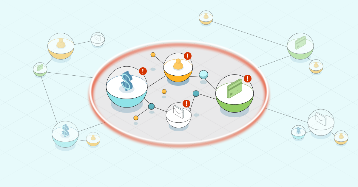
Detect fraud faster with a transaction graph

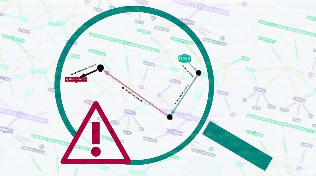
Bolster your cybersecurity by visualizing attack graphs with Neo4j & G.V()