Approximate Maximum K-Cut with Neo4j Graph Data Science

Senior Data Scientist at Neo4j
6 min read

Cluster related products and separate conflicting entities with the newest algorithm in the Graph Data Science Library: Approximate Maximum K-cut

The 1.7 release of Neo4j’s Graph Data Science Library contains some amazing features, like machine learning pipelines for link prediction, and the ability to query in-memory graphs in the graph catalog with Cypher. Amongst all that goodness is a new algorithm called Approximate Maximum K-cut.
The approximate maximum k-cut algorithm will divide a graph into a number of partitions that you specify. The “k” in the algorithm’s name stands for the number of partitions. The goal of the algorithm is to divide the graph in such a way that the sum of the weights of relationships that connect nodes in different partitions is as high as possible.
At first, this struck me as a strange objective for an algorithm. I often think of the relationships in a graph as representing attraction, or similarity. Why would I want to separate things that are similar into different communities?
However, there’s no reason graph relationships can only represent “likes” or “friends.” A relationship could also represent “dislike,” with a weight property that represents the level of mutual antipathy.
Imagine planning a party for guests who haven’t seen each other in a while. Old resentments and lack of recent practice in social interactions might create some awkward moments if you don’t plan the seating at the party’s two tables in a way that separates the most combustible combinations of personalities. Maximum k-cut can help.
To follow the examples in this blog post, you can use a free Neo4j Sandbox. Choose a blank sandbox, because we will add our own data.
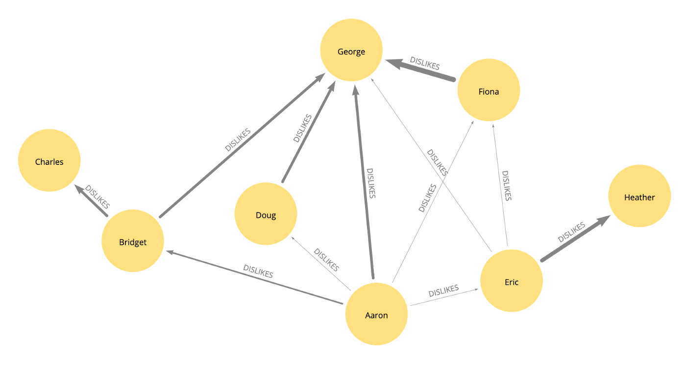
In the Neo4j Browser UI, run this script to create nodes representing party guests (People nodes) and their level of mutual dislike. Even though the relationships are directed, we’ll assume the same level of dislike goes both ways between the parties.
CREATE
(aaron:Person {name: 'Aaron'}),
(bridget:Person {name: 'Bridget'}),
(charles:Person {name: 'Charles'}),
(doug:Person {name: 'Doug'}),
(eric:Person {name: 'Eric'}),
(fiona:Person {name: 'Fiona'}),
(george:Person {name: 'George'}),
(heather:Person {name: 'Heather'}),
(aaron)-[:DISLIKES {strength:2}]->(bridget),
(aaron)-[:DISLIKES {strength:1}]->(doug),
(aaron)-[:DISLIKES {strength:1}]->(eric),
(aaron)-[:DISLIKES {strength:1}]->(fiona),
(aaron)-[:DISLIKES {strength:3}]->(george),
(bridget)-[:DISLIKES {strength:3}]->(charles),
(bridget)-[:DISLIKES {strength:3}]->(george),
(doug)-[:DISLIKES {strength:3}]->(george),
(eric)-[:DISLIKES {strength:1}]->(fiona),
(eric)-[:DISLIKES {strength:1}]->(george),
(eric)-[:DISLIKES {strength:4}]->(heather),
(fiona)-[:DISLIKES {strength:5}]->(george);
I visualized the resulting graph in Neo4j Bloom so that I see the strength property on the relationships as line weight.
Now we’ll create the graph in Neo4j’s in-memory graph catalog.
CALL gds.graph.create(
  'partyGraph',
  'Person',
  {
    DISLIKES: {
      properties: ['strength']
    }
  }
)
Finally, we can use the approximate maximum k-cut algorithm to assign the guests to the two tables.
CALL gds.alpha.maxkcut.stream('partyGraph', {k:2})
YIELD nodeId, communityId
with gds.util.asNode(nodeId) as guest, communityId
return guest.name as name, communityId as tableNumber
order by tableNumber, guest.name

╒═════════╤═════════════╕
│"name"   │"tableNumber"│
╞═════════╪═════════════╡
│"Bridget"│0            │
├─────────┼─────────────┤
│"Doug"   │0            │
├─────────┼─────────────┤
│"Eric"   │0            │
├─────────┼─────────────┤
│"Fiona"  │0            │
├─────────┼─────────────┤
│"Aaron"  │1            │
├─────────┼─────────────┤
│"Charles"│1            │
├─────────┼─────────────┤
│"George" │1            │
├─────────┼─────────────┤
│"Heather"│1            │
└─────────┴─────────────┘
Our seating plan looks promising. There might be some minor tension between Eric and Fiona at table 0, and Aaron and George might create some sparks at table 1. There are no other feuding table-mates to worry about.
The maximum k-cut algorithm has been used for mobile wireless communication planning in a way that reminds me of our dinner party problem. Imagine that instead of assigning table numbers to dinner guests so that incompatible guests don’t share the same table, you want to assign identifiers to cellular towers so that nearby towers’ reference frequencies don’t share the same ID, as described in a paper by Fairbother, Letchford, and Briggs.
A paper by Gaur, Krishnamurti, and Kohli offers some other interesting examples of maximum k-cut in action. I experimented with a retail scenario they suggested. Imagine a bakery that wants to divide its menu into several sections. If items that are frequently purchased together could be clustered in the same menu section, it would increase opportunities for cross-selling.
To explore this scenario, I loaded a bakery-purchases dataset from Kaggle into my Neo4j Sandbox using the steps below.
In Neo4j Browser, I ran these commands to create unique constraints for the node types that will be in my data model.
CREATE CONSTRAINT uniqueTransaction ON (t:Transaction) ASSERT t.ID IS UNIQUE;

CREATE CONSTRAINT uniqueItem ON (i:Item) ASSERT i.name IS UNIQUE;
Then, I ran these commands to load the nodes and relationships.
LOAD CSV WITH HEADERS FROM "https://raw.githubusercontent.com/smithna/datasets/main/bread_basket.csv" AS line
MERGE (t:Transaction {ID:line.Transaction});

LOAD CSV WITH HEADERS FROM "https://raw.githubusercontent.com/smithna/datasets/main/bread_basket.csv" AS line
MERGE (i:Item {name:line.Item});

LOAD CSV WITH HEADERS FROM "https://raw.githubusercontent.com/smithna/datasets/main/bread_basket.csv" AS line
MATCH (t:Transaction {ID:line.Transaction}),
      (i:Item {name:line.Item})
MERGE (t)-[:CONTAINS]->(i);
So far, I had loaded a group of Transaction nodes. Each transaction had a CONTAINS relationship leading to the Item nodes that were purchased in that transaction.
Now, I wanted to know which items did not appear frequently together in the same transactions. It would be good to split these infrequently paired items up into separate sections of the menu.
I counted the total number of transactions in the dataset with this query.
match (t:Transaction) return count(t);

╒══════════╕
│"count(t)"│
╞══════════╡
│9465      │
└──────────┘
Next, I created the GOES_WITH relationship between all possible pairs of items. The relationship has a pairedTransactions property that represent the number of transactions on which the items were both present, and a unpairedTransactions property that represents the number of transactions where one or both of the items were absent.
Keep in mind that if n is the number of items on the menu, the number of pairs to be considered is n * (n-1)/2. That will be an expensive query for large values of n, but it’s fine for the size of our data.
MATCH (i:Item)
WITH collect(i) AS items
WITH apoc.coll.combinations(items, 2, 2) AS pairs
UNWIND pairs AS pair
WITH pair[0] as i0, pair[1] as i1
OPTIONAL MATCH (i0)<-[:CONTAINS]-(t:Transaction)-[:CONTAINS]->(i1)

WITH i0, i1, count(t) AS pairedTransactions

CREATE (i0)-[:GOES_WITH {pairedTransactions:pairedTransactions, unpairedTransactions:9465-pairedTransactions}]->(i1)
Now it was time to create the graph in the Neo4j graph catalog using the “negative” unpairedTransactions weight property.
CALL gds.graph.create(
  'bakeryGraph',
  'Item',
  {
    GOES_WITH: {
      properties: ['unpairedTransactions']
    }
  }
)
I wanted to use the approximate maximum k-cut algorithm to push items with high unpairedTransactions values into separate menu categories. I chose to create 10 different categories. I used this query to modify the in-memory graph with the results of the algorithm run.
CALL gds.alpha.maxkcut.mutate(
  'bakeryGraph',
  {
    mutateProperty: 'menuSection',
    k:10,
    relationshipWeightProperty:'unpairedTransactions',
    concurrency: 1,
    randomSeed: 25
  }
)
YIELD cutCost, nodePropertiesWritten
I wrote the properties from the in-memory graph back to the persistent Neo4j graph.
CALL gds.graph.writeNodeProperties(
  'bakeryGraph',
  ['menuSection']
) YIELD propertiesWritten
Then, I could query the results and see which items ended up in the same menu section.
MATCH (i:Item)<-[:CONTAINS]-(t:Transaction)
RETURN i.menuSection as menuSection, i.name as item, count(t) as transactionCount
ORDER BY menuSection, transactionCount desc

╒═════════════╤═══════════════════════════════╤══════════════════╕
│"menuSection"│"item"                         │"transactionCount"│
╞═════════════╪═══════════════════════════════╪══════════════════╡
│0            │"Soup"                         │326               │
├─────────────┼───────────────────────────────┼──────────────────┤
│0            │"Toast"                        │318               │
├─────────────┼───────────────────────────────┼──────────────────┤
│0            │"Truffles"                     │192               │
├─────────────┼───────────────────────────────┼──────────────────┤
│0            │"Spanish Brunch"               │172               │
├─────────────┼───────────────────────────────┼──────────────────┤
│0            │"Mineral water"                │134               │
├─────────────┼───────────────────────────────┼──────────────────┤
│0            │"Hearty & Seasonal"            │100               │
├─────────────┼───────────────────────────────┼──────────────────┤
It looks like many of the most popular items ended up together in menu section 7.
├─────────────┼───────────────────────────────┼──────────────────┤
│7            │"Coffee"                       │4528              │
├─────────────┼───────────────────────────────┼──────────────────┤
│7            │"Bread"                        │3097              │
├─────────────┼───────────────────────────────┼──────────────────┤
│7            │"Tea"                          │1350              │
├─────────────┼───────────────────────────────┼──────────────────┤
│7            │"Pastry"                       │815               │
├─────────────┼───────────────────────────────┼──────────────────┤
│7            │"Sandwich"                     │680               │
├─────────────┼───────────────────────────────┼──────────────────┤
Customers with a sweet tooth would enjoy section 1 of the menu.
├─────────────┼───────────────────────────────┼──────────────────┤
│1            │"Brownie"                      │379               │
├─────────────┼───────────────────────────────┼──────────────────┤
│1            │"Alfajores"                    │344               │
├─────────────┼───────────────────────────────┼──────────────────┤
│1            │"Coke"                         │184               │
├─────────────┼───────────────────────────────┼──────────────────┤
Several of the non-food items ended up together in section 5.
├─────────────┼───────────────────────────────┼──────────────────┤
│5            │"Tshirt"                       │21                │
├─────────────┼───────────────────────────────┼──────────────────┤
│5            │"Valentine's card"             │13                │
├─────────────┼───────────────────────────────┼──────────────────┤
│5            │"Kids biscuit"                 │12                │
├─────────────┼───────────────────────────────┼──────────────────┤
│5            │"Postcard"                     │10                │
├─────────────┼───────────────────────────────┼──────────────────┤
I hope these examples inspire you to have fun with approximate maximum k-cut as part of your data science toolkit.
Approximate Maximum K-Cut with Neo4j Graph Data Science was originally published in Neo4j Developer Blog on Medium, where people are continuing the conversation by highlighting and responding to this story.
Share Article


Explore
Related Articles


How to Improve Multi-Hop Reasoning With Knowledge Graphs and LLMs