Diversify Your Stock Portfolio with Graph Analytics

Graph ML and GenAI Research, Neo4j
5 min read

A couple of weeks ago, I stumbled upon the stock market volume analysis in Neo4j by Bryant Avey.
Pattern-Driven Insights: Visualize Stock Volume Similarity with Neo4j and Power BI
It got me interested in how we could use graph analytics to analyze stock markets.
After a bit of research, I found this Spread of Risk Across Financial Markets research paper. The authors infer a network between stocks by examining the correlation between stocks and then search for peripheral stocks in the network to help diversifying stock portfolios. As a conclusion of the research paper, the authors argue that this technique could reduce risk by diversifying your investment, and — interestingly — increasing your profits.
Disclaimer: This is not financial advice, and you should do your own research before investing.

We will be using a subset of Kaggle’s NASDAQ-100 Stock Price dataset. The dataset contains price and volume information of 102 securities fro the last decade.
For this post, I have prepared a subset CSV file that contains the stock price and volume information between May and September 2021.
We will use the following graph model to store the stock information:

Each stock ticker will be represented as a separate node. We will store the price and volume information for each stock ticker as a linked list of stock trading days nodes. Using the linked list schema is a general graph model I use when modeling timeseries data in Neo4j.
If you want to follow along with examples in this blog post, I suggest you open a blank project in Neo4j Sandbox.
Neo4j Sandbox provides free cloud instances of Neo4j database that come pre-installed with both the APOC and Graph Data Science plugins. You can copy the following Cypher statement in Neo4j Browser to import the stock information.
:auto USING PERIODIC COMMIT
LOAD CSV WITH HEADERS FROM "https://raw.githubusercontent.com/tomasonjo/blog-datasets/main/stocks/stock_prices.csv" as row

MERGE (s:Stock{name:row.Name})
CREATE (s)-[:TRADING_DAY]->(:StockTradingDay{date: date(row.Date), close:toFloat(row.Close), volume: toFloat(row.Volume)});
Next, we need to create a linked list between stock trading days nodes. We can easily create a linked list with the apoc.nodes.link procedure. We will also collect the closing prices by days of stocks and store them as a list property of the stock node.
MATCH (s:Stock)-[:TRADING_DAY]->(day)
WITH s, day
ORDER BY day.date ASC
WITH s, collect(day) as nodes, collect(day.close) as closes
SET s.close_array = closes
WITH nodes
CALL apoc.nodes.link(nodes, 'NEXT_DAY')
RETURN distinct 'done' AS result
Here is a sample linked list visualization in Neo4j Browser:

Inferring relationships based on the correlation coefficient
We will use the Pearson similarity as the correlation metric. The authors of the above-mentioned research paper use more sophisticated correlation metrics, but that is beyond the scope of this blog post.
The input to the Pearson similarity algorithm will be the ordered list of closing prices we produced in the previous step. The algorithm will calculate the correlation coefficient and store the results as relationships between most correlating stocks. I have used the topKparameter value of 3, so each stock will be connected to the three most correlating stock tickers.
MATCH (s:Stock)
WITH {item:id(s), weights: s.close_array} AS stockData
WITH collect(stockData) AS input
CALL gds.alpha.similarity.pearson.write({
  data: input,
  topK: 3,
  similarityCutoff: 0.2
})
YIELD nodes, similarityPairs
RETURN nodes, similarityPairs
As mentioned, the algorithm produced new SIMILAR relationships between stock ticker nodes.

We can now run a community detection algorithm to identify various clusters of correlating stocks. I have decided to use the Louvain Modularity in this example. The community ids will be stored as node properties.
CALL gds.louvain.write({
  nodeProjection:'Stock',
  relationshipProjection:'SIMILAR',
  writeProperty:'louvain'
})
With such small graphs, I find the best way to examine community detection results is to simply produce a network visualization.

I won’t go into much detail explaining the community structure of the visualization, as we only looked at three months period for 100 stock tickers.
Following the research paper idea, you would want to invest in stocks from different communities to diversify your risk and increase profits. You could pick the stocks from each community using a linear regression slope to indicate their performance.
I found there is a simple linear regression model available as an apoc.math.regr procedure. Read more about it in the documentation. Unfortunately, the developers had different data model in mind for performing linear regression, so we first have to adjust the graph model to fit the procedure input. In the first step, we add a secondary label to the stock trading days nodes that indicate the stock ticker it represents.
MATCH (s:Stock)-[:TRADING_DAY]->(day)
CALL apoc.create.addLabels( day, [s.name]) YIELD node
RETURN distinct 'done'
Next, we need to calculate the x-axis index values. We will simply assign an index value of zero to each stock’s first trading day and increment the index value for each subsequent trading day.
MATCH (s:Stock)-[:TRADING_DAY]->(day)
WHERE NOT ()-[:NEXT_DAY]->(day)
MATCH p=(day)-[:NEXT_DAY*0..]->(next_day)
SET next_day.index = length(p)
Now that our graph model fits the linear regression procedure in APOC, we can go ahead and calculate the slope value of the fitted line. In a more serious setting, we would probably want to scale the closing prices, but we will skip it for this demonstration. The slope value will be stored as a node property.
MATCH (s:Stock)
CALL apoc.math.regr(s.name, 'close', 'index') YIELD slope
SET s.slope = slope;
As a last step, we can recommend the top three performing stocks from each community.
MATCH (s:Stock)
WITH s.louvain AS community, s.slope AS slope, s.name AS ticker
ORDER BY slope DESC
RETURN community, collect(ticker)[..3] as potential_investments
Results
Conclusion
This is not financial advice — do your own research before investing. Even so, in this blog post, I only looked at a 90-day window for NASDAQ-100 stocks, where the markets were doing well, so the results might not be that great in diversifying your risk.
If you want to get more serious, you would probably want to collect a more extensive dataset and fine-tune the correlation coefficient calculation. Not only that, but a simple linear regression might not be the best indicator of stock performance.
You can start with your graph analysis today and skip the environment configuration hassle by using the free Neo4j Sandbox instances. Let me know how your approach turned out!
As always, the code is available on GitHub.
Diversify Your Stock Portfolio with Graph Analytics was originally published in Neo4j Developer Blog on Medium, where people are continuing the conversation by highlighting and responding to this story.
Share Article


Explore
Related Articles

Text2Cypher Across Languages: Evaluating Foundational Models Beyond English