Hot algo summer: New algorithms in Neo4j Graph Data Science

Developer Advocate, Neo4j
13 min read


Rev up your graph algorithm game with these hot new offerings
Summer is heating up, and so is the world of graph algorithms! Neo4j Graph Data Science has just unleashed a collection of innovative algorithms that can solve some pain points. Have you been struggling with how to include negative weights in your pathfinding? Are you more interested in community detection that identifies central and peripheral clusters based on a given density? Or maybe you can’t seem to get a good sample of a large graph. Prepare to be pleased as we take a closer look at the underlying methodologies of these exciting additions: K-Core Decomposition, Bellman-Ford shortest path algorithm, and Common Neighbour Aware Random Walk (CNARW). With these scorching new tools in your arsenal, get ready to take on complex graph analysis tasks and uncover extraordinary insights. Don’t let your algorithms simmer this summer — turn up the heat and make the most of these hot new offerings!
K-core decomposition
Enhanced flexibility and precision in community detection
The K-Core Decomposition algorithm, available in Neo4j Graph Data Science 2.4, is based on the concept of partitioning a graph into layers, progressing from peripheral to central nodes. It recursively identifies subgraphs where each node has at least k connections, with k ranging from 0 to the maximum degree of the graph.
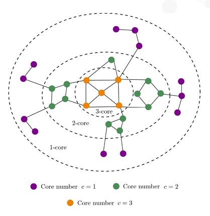
K-Core Decomposition allows users to easily analyze community structures and identify influential nodes, providing a flexible and granular approach for community detection in social networks, protein-protein interactions in drug discovery, and optimizing information spreading in network design. This algorithm can be particularly useful if you have communities of varying density or are interested in the granularity of the connectivity level of each node. See the Code Example below.
Bellman-Ford shortest path
Native support for negative weights and comprehensive analytics
The Bellman-Ford shortest path algorithm, introduced in Graph Data Science 2.4, enables the calculation of the shortest paths in graphs, even with negative weights. The improved version, Shortest-Path Faster Algorithm (SPFA), employs sampling and parallelization techniques to significantly reduce computation time.
This algorithm is particularly useful in IT networking for tasks such as routing, load balancing, analyzing network topology, and optimizing costs. In supply chain optimization and finance, the Bellman-Ford algorithm enables efficient resource allocation and routing decisions by considering the weight of edges along the path. If you have been struggling with how to manage negative weights, Bellman-Ford is a must-try. Code Example
Common neighbour aware random walk (CNARW)
Integration for efficient subgraph sampling
The Common Neighbour Aware Random Walk (CNARW) algorithm, introduced in Graph Data Science 2.4, is a graph sampling technique that helps scale machine learning on large graphs. Sampling large graphs has inherent challenges. Are the samples coming from different clusters? Are structures and attributes represented in the sample? How do you maintain the key structural aspects of the graph yet keep the sample a manageable size? CNARW and its cross-cluster approach do just this.
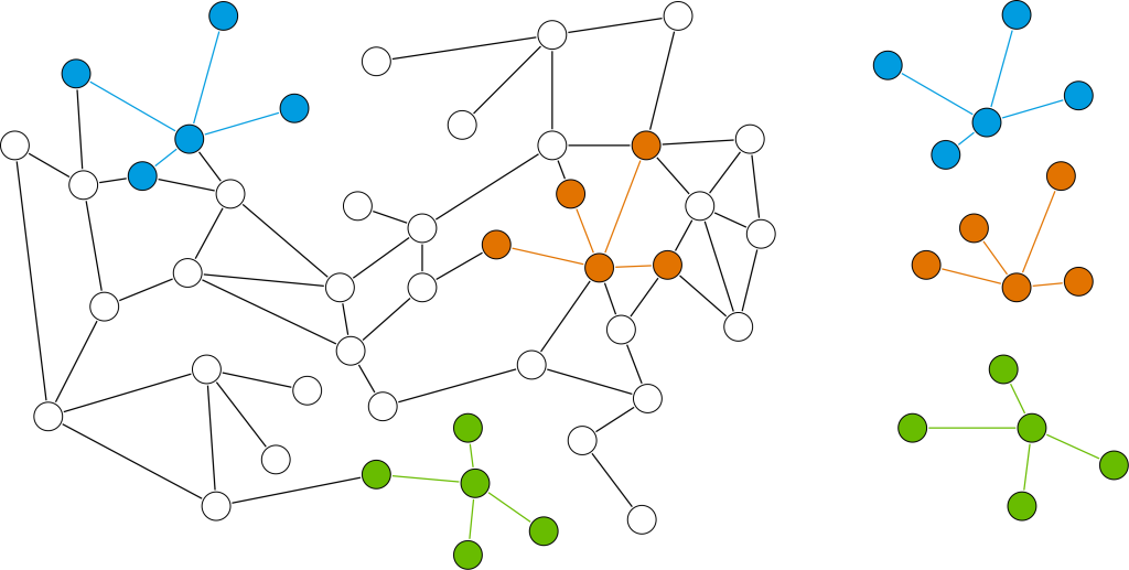
By considering the common neighbors of nodes, CNARW decreases the odds of sampling duplicate nodes. This improves the representativeness of the sampled subgraphs and reduces bias towards densely connected regions, resulting in a more accurate and balanced representation of the graph’s structure. CNARW finds applications in recommendation engines, anomaly detection, and market segmentation by suggesting items of interest based on common neighbors, identifying deviant nodes, and effectively identifying densely connected groups of nodes that correspond to communities. Code Example
With the introduction of K-Core Decomposition, Bellman-Ford shortest path algorithm (SPFA), and Common Neighbour Aware Random Walk (CNARW) in Graph Data Science 2.4, Neo4j allows Data Scientists to expand your algorithmic toolbox and refine the ability to find the right algorithm for the right problem.
To stay up to date on all things Graph Data Science, check out our What’s New, listen to our podcast, or connect with me on LinkedIn. I’m always interested in content requests, so reach out!
Code examples
All code snippets are written in Cypher.
K-core decomposition
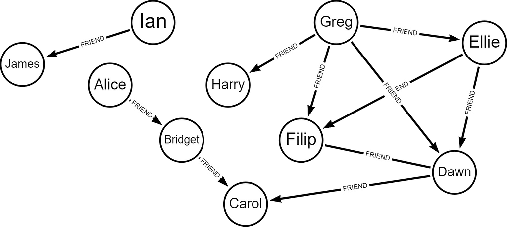
Let’s say we have a graph of friends.
CREATE (alice:User {name: ‘Alice’}),
(bridget:User {name: ‘Bridget’}),
(charles:User {name: ‘Charles’}),
(doug:User {name: ‘Doug’}),
(eli:User {name: ‘Eli’}),
(filip:User {name: ‘Filip’}),
(greg:User {name: ‘Greg’}),
(harry:User {name: ‘Harry’}),
(ian:User {name: ‘Ian’}),
(james:User {name: ‘James’}),
(alice)-[:FRIEND]->(bridget),
(bridget)-[:FRIEND]->(charles),
(charles)-[:FRIEND]->(doug),
(charles)-[:FRIEND]->(harry),
(doug)-[:FRIEND]->(eli),
(doug)-[:FRIEND]->(filip),
(doug)-[:FRIEND]->(greg),
(eli)-[:FRIEND]->(filip),
(eli)-[:FRIEND]->(greg),
(filip)-[:FRIEND]->(greg),
(greg)-[:FRIEND]->(harry),
(ian)-[:FRIEND]->(james)
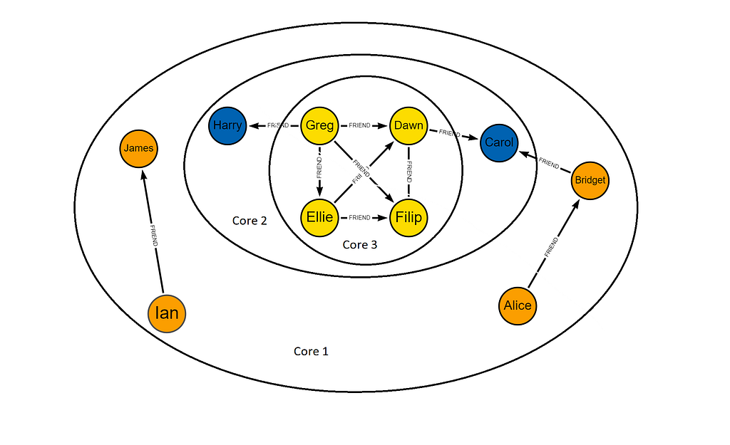
Start by creating a projection of the graph called ‘graph’ based on the node label type ‘User’ with relationship of FRIEND undirected.
CALL gds.graph.project('graph', 'User', {FRIEND: {orientation: 'UNDIRECTED'}})
Now you can run the K-Core Decomposition on this projection.
CALL gds.kcore.stream(
     graphName: String,
     configuration: Map)
YIELD nodeId: Integer,
      coreValue: Float
Because we used the stream function, the following results will be returned.
+ — — — — — — -+ — — — — — -+
| name         | coreValue  |
+ — — — — — — -+ — — — — — -+
| “James”      |     1      |
| “Ian”        |     1      |
| “Bridget”    |     1      |
| “Alice”      |     1      |
| “Harry”      |     2      |
| “Charles”    |     2      |
| “Greg”       |     3      |
| “Filip”      |     3      |
| “Eli”        |     3      |
| “Doug”       |     3      |
+ — — — — — — -+ — — — — — -+
You can see when we visualize the core assignments, the most densely connected nodes are in the center. Cores are assigned from the most peripheral to the innermost core.
For more information on writing these results to your database or mutating your projected graph check out the documentation.
_________________________________________________________________
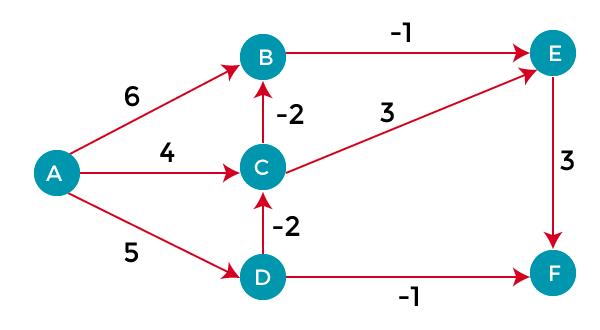
Bellman-Ford shortest path
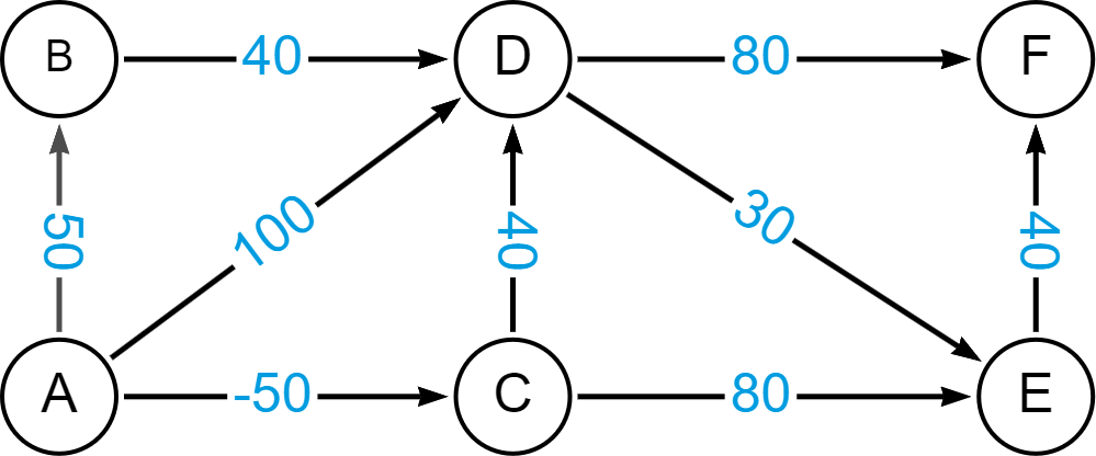
Let’s create a graph with relationships having a weight property “cost” between nodes. The cost property can be either positive or negative.
CREATE (a:Node {name: ‘A’}),
  (b:Node {name: ‘B’}),
  (c:Node {name: ‘C’}),
  (d:Node {name: ‘D’}),
  (e:Node {name: ‘E’}),
  (f:Node {name: ‘F’}),
  (g:Node {name: ‘G’}),
  (h:Node {name: ‘H’}),
  (i:Node {name: ‘I’}),
  (a)-[:REL {cost: 50}]->(b),
  (a)-[:REL {cost: -50}]->(c),
  (a)-[:REL {cost: 100}]->(d),
  (b)-[:REL {cost: 40}]->(d),
  (c)-[:REL {cost: 40}]->(d),
  (c)-[:REL {cost: 80}]->(e),
  (d)-[:REL {cost: 30}]->(e),
  (d)-[:REL {cost: 80}]->(f),
  (e)-[:REL {cost: 40}]->(f),
  (g)-[:REL {cost: 40}]->(h),
  (h)-[:REL {cost: -60}]->(i),
  (i)-[:REL {cost: 10}]->(g)
Graph Data Science algorithms are run on projections, so let’s first create a projection.
CALL gds.graph.project( ‘myGraph’,
                        ‘Node’,
                        ‘REL’, { relationshipProperties: ‘cost’ } )
The Bellman-Ford Single Source algorithm calculates the shortest path based on the chosen weight. In this case, we are weighting the paths by the relationship labeled ‘REL’ on the property ‘cost’. Let’s find out the shortest paths from a single source node “A”. We want to be able to see each shortest path and its total cost, so let’s expand the YIELD and RETURN statements to include these values and stream the outputs.
MATCH (source:Node {name: ‘A’})

CALL gds.bellmanFord.stream(‘myGraph’,
                            { sourceNode: source,
                              relationshipWeightProperty: ‘cost’ })

YIELD index,
      sourceNode,
      targetNode,
      totalCost,
      nodeIds,
      costs,
      isNegativeCycle

RETURN index,
      gds.util.asNode(sourceNode).name AS source,
      gds.util.asNode(targetNode).name AS target,
      totalCost,
      [nodeId IN nodeIds | gds.util.asNode(nodeId).name] AS nodeNames,
      costs,
      isNegativeCycle as isNegativeCycle

ORDER BY index
NB: We include the output ‘isNegativeCycle’ to determine if there is a path from source back to source that is negative in cost. If so, the path can be traversed many times making the cost smaller and smaller, therefore these would be noted if they exist.
The results for shortest paths based on “cost” from A to each possible node will be as follows.
+ — — — -+ — — — — — — + — — — — — — + — — — — — -+ — — — — — — — — -+ — — — — — — — — — — — — -+ —
| Index | source| target | totalCost | nodeNames       | costs                   | isNegativeCycle |
+ — — — -+ — — — — — — + — — — — — — + — — — — — -+ — — — — — — — — -+ — — — — — — — — — — + — — —+
| 0     | “A”   |   “A”  | 0.0       | [A]             | [0]                     | false           |
| 1     | “A”   |   “B”  | 50.0      | [A, B]          | [0, 50]                 | false           |
| 2     | “A”   |   “C”  | -50.0     | [A, C]          | [0, -50]                | false           |
| 3     | “A”   |   “D”  | -10.0     | [A, C, D]       | [0, -50, -10]           | false           |
| 4     | “A”   |   “E”  | 20.0      | [A, C, D, E]    | [0, -50, -10, 20] |     | false           |
| 5     | “A”   |   “F”  | 60.0      | [A, C, D, E, F] | [0, -50, -10.0, 20, 60] | false           |
+ — — — -+ — — — — — — + — — — — — — + — — — — — -+ — — — — — — — — -+ — — — — — — — — — - + - - -+
What you will note in these paths is that what may be considered the shortest path if you were using number of hops as the criteria will not be so in the case of Bellman-Ford. Let’s look at the shortest path from A to F. If not, considering the cost, one would think the path A->D->F would be the shortest path. We see below, however, that A->D->F would have a cost of 180, whereas A->C->D->E->F has a total cost of only 60.
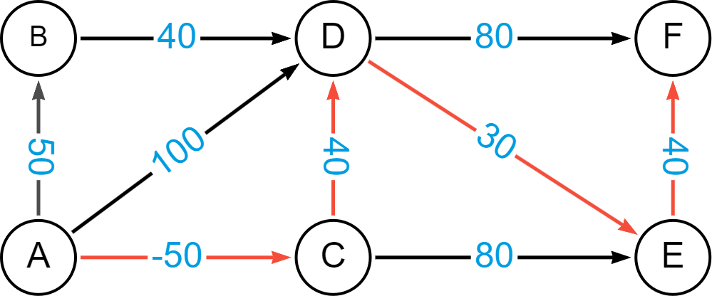
You can see clearly how having an algorithm such as Bellman-Ford can enable better pathfinding when leveraging negative weights.
_________________________________________________________________
Common neighbour aware random walk (CNARW)
Let’s take a look at a small sample of characters from Romeo & Juliet.
CREATE
 (J:female {id:’Juliette’}),
 (R:male {id:’Romeo’}),
 (r1:male {id:’Ryan’}),
 (r2:male {id:’Robert’}),
 (r3:male {id:’Riley’}),
 (r4:female {id:’Ruby’}),
 (j1:female {id:’Josie’}),
 (j2:male {id:’Joseph’}),
 (j3:female {id:’Jasmine’}),
 (j4:female {id:’June’}),
 (J)-[:LINK]->(R), (R)-[:LINK]->(J),
 (r1)-[:LINK]->(R), (R)-[:LINK]->(r1), (r2)-[:LINK]->(R), (R)-[:LINK]->(r2),
 (r3)-[:LINK]->(R), (R)-[:LINK]->(r3), (r4)-[:LINK]->(R), (R)-[:LINK]->(r4),
 (r1)-[:LINK]->(r2), (r2)-[:LINK]->(r1), (r1)-[:LINK]->(r3), (r3)-[:LINK]->(r1),
 (r1)-[:LINK]->(r4), (r4)-[:LINK]->(r1), (r2)-[:LINK]->(r3), (r3)-[:LINK]->(r2),
 (r2)-[:LINK]->(r4), (r4)-[:LINK]->(r2), (r3)-[:LINK]->(r4), (r4)-[:LINK]->(r3),
 (j1)-[:LINK]->(J), (J)-[:LINK]->(j1), (j2)-[:LINK]->(J), (J)-[:LINK]->(j2),
 (j3)-[:LINK]->(J), (J)-[:LINK]->(j3), (j4)-[:LINK]->(J), (J)-[:LINK]->(j4),
 (j1)-[:LINK]->(j2), (j2)-[:LINK]->(j1), (j1)-[:LINK]->(j3), (j3)-[:LINK]->(j1),
 (j1)-[:LINK]->(j4), (j4)-[:LINK]->(j1), (j2)-[:LINK]->(j3), (j3)-[:LINK]->(j2),
 (j2)-[:LINK]->(j4), (j4)-[:LINK]->(j2), (j3)-[:LINK]->(j4), (j4)-[:LINK]->(j3) ;
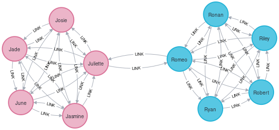
Neo4j algorithms are run on projections of the graph. Let’s create that projection.
CALL gds.graph.project( ‘myGraph’, [‘male’, ‘female’], ‘LINK’ )
Now we can go ahead and sample the graph. The parameter ‘sampling ratio’ represents the portion of the graph you want in each sample. In this case, we created a graph with 10 nodes. Let’s say we want the random sample to contain 5 nodes,we would set the sampling ratio to 5/10 or .5. Obviously, the intention is to sample a large graph, so this number will be significantly smaller in a real-world scenario.
MATCH (start:female {id: ‘Juliette’})

CALL gds.graph.sample.cnarw(‘mySampleCNARW’, ‘myGraph’,
        { samplingRatio: 0.5,
          startNodes: [id(start)] })

YIELD nodeCount

RETURN nodeCount
This number on the output will vary, given that the walks are random. In this case, the output was as follows.
+ — — — — — -+
| nodeCount  |
+ — — — — — -+
|     5      |
+ — — — — — -+
The main difference between the Common Neighbour Aware Random Walk and other random walk sampling is that there are more chances to go into another cluster rather than getting caught in a local area. By choosing a node with a higher degree and fewer common neighbors with previously visited nodes (or the current node)chances of discovering unvisited nodes are increased but the probability of revisiting previously visited nodes in future steps is reduced.
Hot Algo Summer was originally published in Neo4j Developer Blog on Medium, where people are continuing the conversation by highlighting and responding to this story.
Share Article


Explore
Related Articles


SumoDB in Neo4j: Chaining Multiple Graph Algorithms in Snowflake — Part 3