Integrating Microsoft GraphRAG Into Neo4j

Graph ML and GenAI Research, Neo4j
22 min read
Store the MSFT GraphRAG output into Neo4j and implement local and global retrievers with LangChain or LlamaIndex
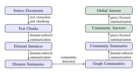
Microsoft’s GraphRAG implementation has gained significant attention lately. In my last blog post, I discussed how the graph is constructed and explored some of the innovative aspects highlighted in the research paper. At a high level, the input to the GraphRAG library are source documents containing various information. The documents are processed using an Large Language Model (LLM) to extract structured information about entities appearing in the documents along with their relationships. This extracted structured information is then used to construct a knowledge graph.
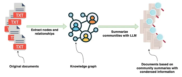
High-level indexing pipeline as implemented in the GraphRAG paper by Microsoft — Image by author
After the knowledge graph has been constructed, the GraphRAG library uses a combination of graph algorithms, specifically Leiden community detection algorithm, and LLM prompting to generate natural language summaries of communities of entities and relationships found in the knowledge graph.
In this post, we’ll take the output from the GraphRAG library, store it in Neo4j, and then set up retrievers directly from Neo4j using LangChain and LlamaIndex orchestration frameworks.
The code and GraphRAG output are accessible on GitHub, allowing you to skip the GraphRAG extraction process.
Dataset
The dataset featured in this blog post is “A Christmas Carol” by Charles Dickens, which is freely accessible via the Gutenberg Project.
A Christmas Carol by Charles Dickens
We selected this book as the source document because it is highlighted in the introductory documentation, allowing us to perform the extraction effortlessly.
Graph Construction
Even though you can skip the graph extraction part, we’ll talk about a couple of configuration options I think are the most important. For example, graph extraction can be very token-intensive and costly. Therefore, testing the extraction with a relatively cheap but good-performing LLM like gpt-4o-mini makes sense. The cost reduction from gpt-4-turbo can be significant while retaining good accuracy, as described in this blog post.
GRAPHRAG_LLM_MODEL=gpt-4o-miniThe most important configuration is the type of entities we want to extract. By default, organizations, people, events, and geo are extracted.
GRAPHRAG_ENTITY_EXTRACTION_ENTITY_TYPES=organization,person,event,geoThese default entity types might work well for a book, but make sure to change them accordingly to the domain of the documents you are looking at processing for a given use case.
Another important configuration is the max gleanings value. The authors identified, and we also validated separately, that an LLM doesn’t extract all the available information in a single extraction pass.
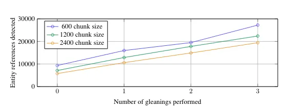
Number of extract entities given the size of text chunks — Image from the GraphRAG paper, licensed under CC BY 4.0
The gleaning configuration allows the LLM to perform multiple extraction passes. In the above image, we can clearly see that we extract more information when performing multiple passes (gleanings). Multiple passes are token-intensive, so a cheaper model like gpt-4o-mini helps to keep the cost low.
GRAPHRAG_ENTITY_EXTRACTION_MAX_GLEANINGS=1Additionally, the claims or covariate information is not extracted by default. You can enable it by setting the GRAPHRAG_CLAIM_EXTRACTION_ENABLED configuration.
GRAPHRAG_CLAIM_EXTRACTION_ENABLED=False
GRAPHRAG_CLAIM_EXTRACTION_MAX_GLEANINGS=1
It seems that it’s a recurring theme that not all structured information is extracted in a single pass. Hence, we have the gleaning configuration option here as well.
What’s also interesting, but I haven’t had time to dig deeper is the prompt tuning section. Prompt tuning is optional, but highly encouraged as it can improve accuracy.
After the configuration has been set, we can follow the instructions to run the graph extraction pipeline, which consists of the following steps.
Steps in the pipeline — Image from the GraphRAG paper, licensed under CC BY 4.0
The extraction pipeline executes all the blue steps in the above image. Review my previous blog post to learn more about graph construction and community summarization. The output of the graph extraction pipeline of the MSFT GraphRAG library is a set of parquet files, as shown in the Operation Dulce example.
These parquet files can be easily imported into the Neo4j graph database for downstream analysis, visualization, and retrieval. We can use a free cloud Aura instance or set up a local Neo4j environment. My friend Michael Hunger did most of the work to import the parquet files into Neo4j. We’ll skip the import explanation in this blog post, but it consists of importing and constructing a knowledge graph from five or six CSV files. If you want to learn more about CSV importing, you can check the Neo4j Graph Academy course.
The import code is available as a Jupyter notebook on GitHub along with the example GraphRAG output.
blogs/msft_graphrag/ms_graphrag_import.ipynb at master · tomasonjo/blogs
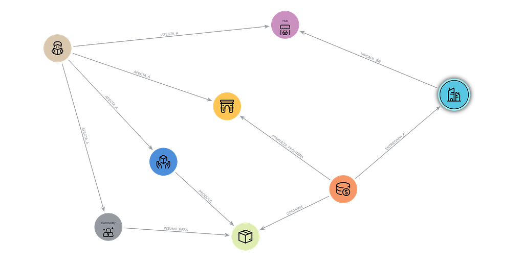
After the import is completed, we can open the Neo4j Browser to validate and visualize parts of the imported graph.
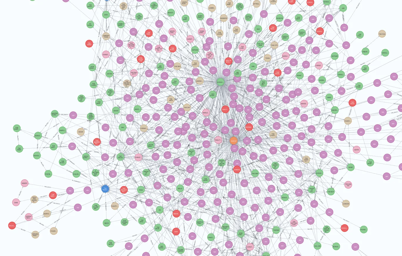
Part of the imported graph. Image by the author.
Graph Analysis
Before moving onto retriever implementation, we’ll perform a simple graph analysis to familiarize ourselves with the extracted data. We start by defining the database connection and a function that executes a Cypher statement (graph database query language) and outputs a Pandas DataFrame.
NEO4J_URI="bolt://localhost"
NEO4J_USERNAME="neo4j"
NEO4J_PASSWORD="password"

driver = GraphDatabase.driver(NEO4J_URI, auth=(NEO4J_USERNAME, NEO4J_PASSWORD))

def db_query(cypher: str, params: Dict[str, Any] = {}) -> pd.DataFrame:
    """Executes a Cypher statement and returns a DataFrame"""
    return driver.execute_query(
        cypher, parameters_=params, result_transformer_=Result.to_df
    )
When performing the graph extraction, we used a chunk size of 300. Since then, the authors have changed the default chunk size to 1200. We can validate the chunk sizes using the following Cypher statement.
db_query(
  "MATCH (n:__Chunk__) RETURN n.n_tokens as token_count, count(*) AS count"
)
# token_count count
# 300         230
# 155         1
230 chunks have 300 tokens, while the last one has only 155 tokens. Let’s now check an example entity and its description.
db_query(
  "MATCH (n:__Entity__) RETURN n.name AS name, n.description AS description LIMIT 1"
)
Results
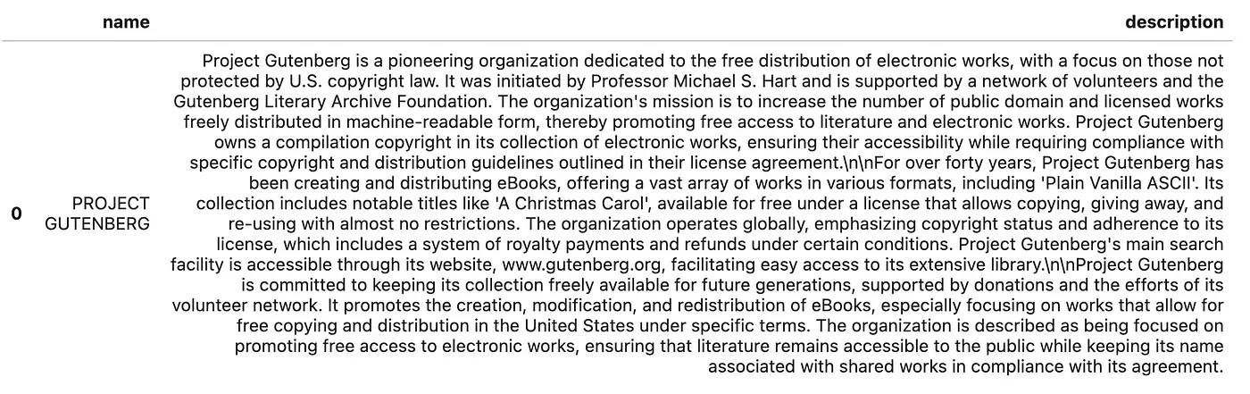
Example entity name and description. Image by author.
It seems that the project Gutenberg is described in the book somewhere, probably at the beginning. We can observe how a description can capture more detailed and intricate information than just an entity name, which the MSFT GraphRAG paper introduced to retain more sophisticated and nuanced data from text.
Let’s check example relationships as well.
db_query(
  "MATCH ()-[n:RELATED]->() RETURN n.description AS description LIMIT 5"
)
Results
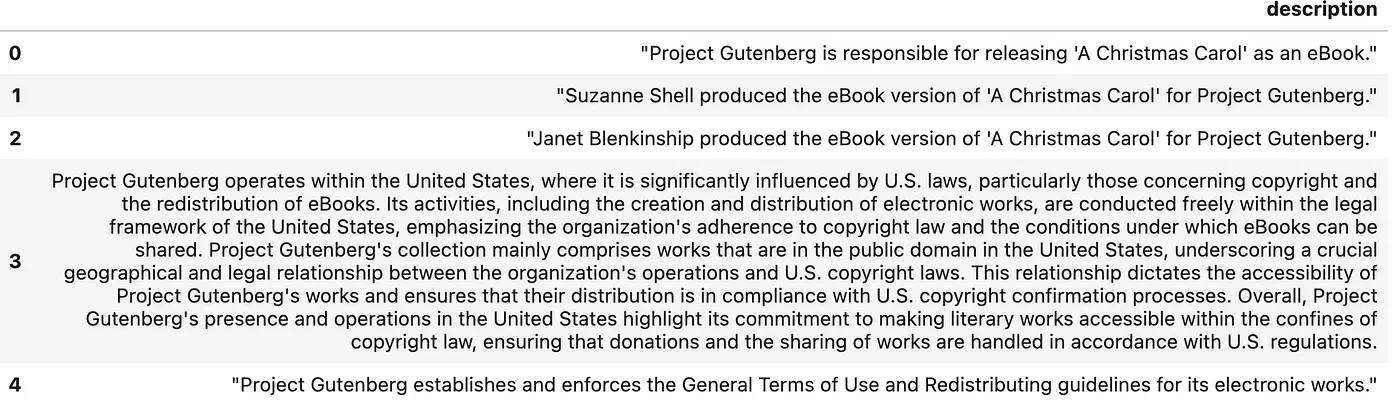
Example relationship descriptions. Image by author.
The MSFT GraphRAG goes beyond merely extracting simple relationship types between entities by capturing detailed relationship descriptions. This capability allows it to capture more nuanced information than straightforward relationship types.
We can also examine a single community and its generated descriptions.
db_query("""
  MATCH (n:__Community__)
  RETURN n.title AS title, n.summary AS summary, n.full_content AS full_content LIMIT 1
""")
Results
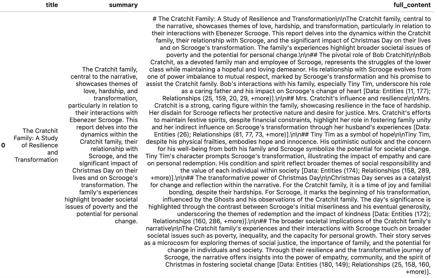
Example community description. Image by author.
A community has a title, summary, and full content generated using an LLM. I haven’t seen if the authors use the full context or just the summary during retrieval, but we can choose between the two. We can observe citations in the full_content, which point to entities and relationships from which the information came. It’s funny that an LLM sometimes trims the citations if they are too long, like in the following example.
[Data: Entities (11, 177); Relationships (25, 159, 20, 29, +more)]There is no way to expand the +more sign, so this is a funny way of dealing with long citations by an LLM.
Let’s now evaluate some distributions. We’ll start by inspecting the distribution of the count of extracted entities from text chunks.
entity_df = db_query(
    """
MATCH (d:__Chunk__)
RETURN count {(d)-[:HAS_ENTITY]->()} AS entity_count
"""
)
# Plot distribution
plt.figure(figsize=(10, 6))
sns.histplot(entity_df['entity_count'], kde=True, bins=15, color='skyblue')
plt.axvline(entity_df['entity_count'].mean(), color='red', linestyle='dashed', linewidth=1)
plt.axvline(entity_df['entity_count'].median(), color='green', linestyle='dashed', linewidth=1)
plt.xlabel('Entity Count', fontsize=12)
plt.ylabel('Frequency', fontsize=12)
plt.title('Distribution of Entity Count', fontsize=15)
plt.legend({'Mean': entity_df['entity_count'].mean(), 'Median': entity_df['entity_count'].median()})
plt.show()
Results
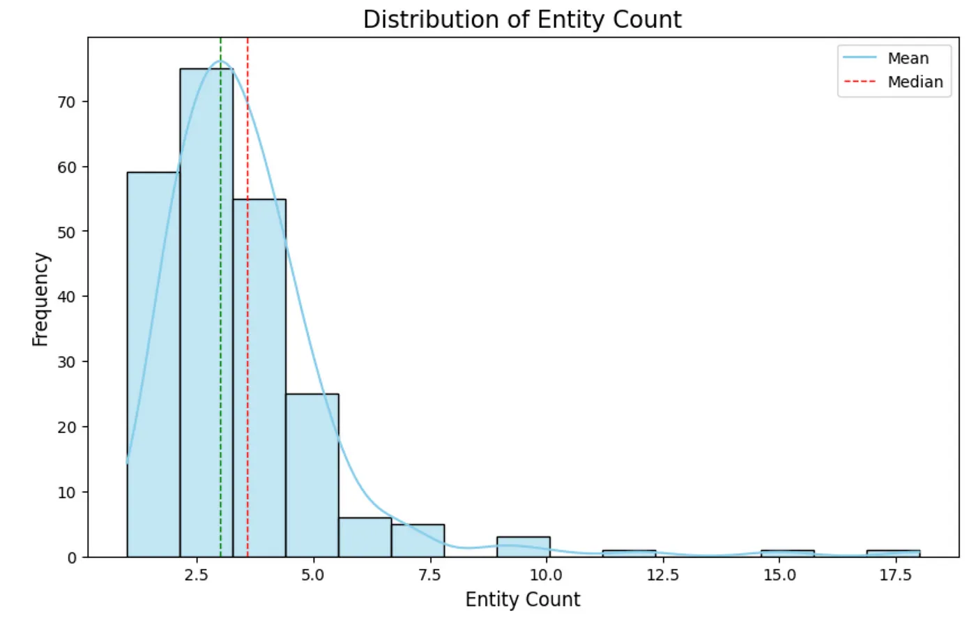
Distribution of the count of extracted entities from text chunks. Image by author.
Remember, text chunks have 300 tokens. Therefore, the number of extracted entities is relatively small, with an average of around three entities per text chunk. The extraction was done without any gleanings (a single extraction pass). It would be interesting to see the distribution if we increased the gleaning count.
Next, we will evaluate the node degree distribution. A node degree is the number of relationships a node has.
degree_dist_df = db_query(
    """
MATCH (e:__Entity__)
RETURN count {(e)-[:RELATED]-()} AS node_degree
"""
)
# Calculate mean and median
mean_degree = np.mean(degree_dist_df['node_degree'])
percentiles = np.percentile(degree_dist_df['node_degree'], [25, 50, 75, 90])
# Create a histogram with a logarithmic scale
plt.figure(figsize=(12, 6))
sns.histplot(degree_dist_df['node_degree'], bins=50, kde=False, color='blue')
# Use a logarithmic scale for the x-axis
plt.yscale('log')
# Adding labels and title
plt.xlabel('Node Degree')
plt.ylabel('Count (log scale)')
plt.title('Node Degree Distribution')
# Add mean, median, and percentile lines
plt.axvline(mean_degree, color='red', linestyle='dashed', linewidth=1, label=f'Mean: {mean_degree:.2f}')
plt.axvline(percentiles[0], color='purple', linestyle='dashed', linewidth=1, label=f'25th Percentile: {percentiles[0]:.2f}')
plt.axvline(percentiles[1], color='orange', linestyle='dashed', linewidth=1, label=f'50th Percentile: {percentiles[1]:.2f}')
plt.axvline(percentiles[2], color='yellow', linestyle='dashed', linewidth=1, label=f'75th Percentile: {percentiles[2]:.2f}')
plt.axvline(percentiles[3], color='brown', linestyle='dashed', linewidth=1, label=f'90th Percentile: {percentiles[3]:.2f}')
# Add legend
plt.legend()
# Show the plot
plt.show()
Results
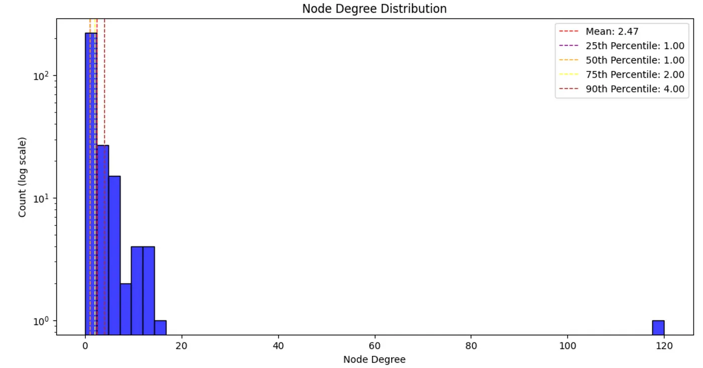
Node degree distribution. Image by author.
Most real-world networks follow a power-law node degree distribution, with most nodes having relatively small degrees and some important nodes having a lot. While our graph is small, the node degree follows the power law. It would be interesting to identify which entity has 120 relationships (connected to 43% of entities).
db_query("""
  MATCH (n:__Entity__)
  RETURN n.name AS name, count{(n)-[:RELATED]-()} AS degree
  ORDER BY degree DESC LIMIT 5""")
Results
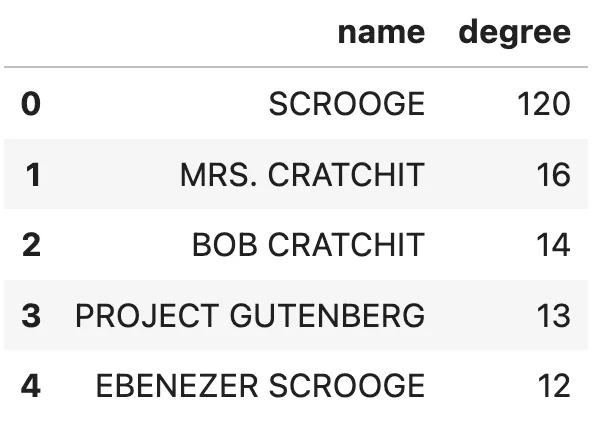
Entities with the most relationships. Image by author.
Without any hesitation, we can assume that Scrooge is the book’s main character. I would also venture a guess that Ebenezer Scrooge and Scrooge are actually the same entity, but as the MSFT GraphRAG lacks an entity resolution step, they weren’t merged.
It also shows that analyzing and cleaning the data is a vital step to reducing noise information, as Project Gutenberg has 13 relationships, even though they are not part of the book story.
Lastly, we’ll inspect the distribution of community size per hierarchical level.
community_data = db_query("""
  MATCH (n:__Community__)
  RETURN n.level AS level, count{(n)-[:IN_COMMUNITY]-()} AS members
""")

stats = community_data.groupby('level').agg(
    min_members=('members', 'min'),
    max_members=('members', 'max'),
    median_members=('members', 'median'),
    avg_members=('members', 'mean'),
    num_communities=('members', 'count'),
    total_members=('members', 'sum')
).reset_index()

# Create box plot
plt.figure(figsize=(10, 6))
sns.boxplot(x='level', y='members', data=community_data, palette='viridis')
plt.xlabel('Level')
plt.ylabel('Members')

# Add statistical annotations
for i in range(stats.shape[0]):
    level = stats['level'][i]
    max_val = stats['max_members'][i]
    text = (f"num: {stats['num_communities'][i]}n"
            f"all_members: {stats['total_members'][i]}n"
            f"min: {stats['min_members'][i]}n"
            f"max: {stats['max_members'][i]}n"
            f"med: {stats['median_members'][i]}n"
            f"avg: {stats['avg_members'][i]:.2f}")
    plt.text(level, 85, text, horizontalalignment='center', fontsize=9)

plt.show()
Results
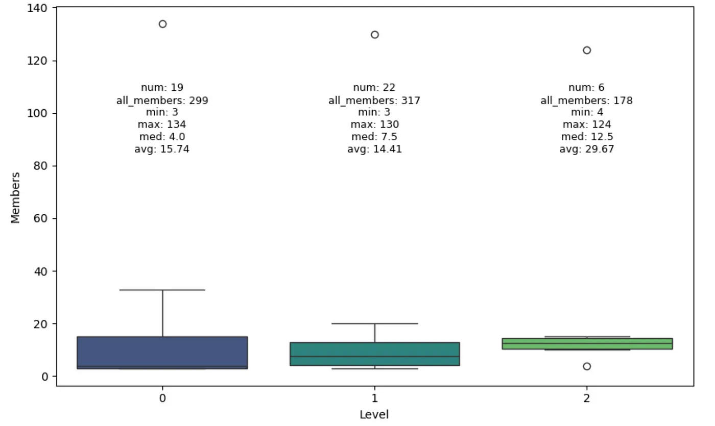
Community size distribution per level. Image by author.
The Leiden algorithm identified three levels of communities, where the communities on higher levels are larger on average. However, there are some technical details that I’m not aware of because if you check the all_members count, and you can see that each level has a different number of all nodes, even though they should be the same in theory. Also, if communities merge at higher levels, why do we have 19 communities on level 0 and 22 on level 1? The authors have done some optimizations and tricks here, which I haven’t had a time to explore in detail yet.
Read a complimentary Gartner® report on knowledge graphs for AI
Implementing Retrievers
In the last part of this blog post, we will discuss the local and global retrievers as specified in the MSFT GraphRAG. The retrievers will be implemented and integrated with LangChain and LlamaIndex.
Local Retriever
The local retriever starts by using vector search to identify relevant nodes, and then collects linked information and injects it into the LLM prompt.
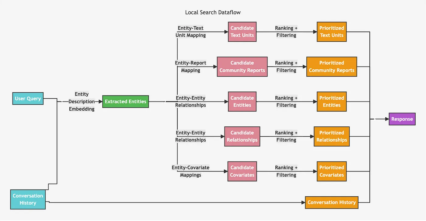
Local retriever architecture. Image from https://microsoft.github.io/graphrag/posts/query/1-local_search/
While this diagram might look complex, it can be easily implemented. We start by identifying relevant entities using a vector similarity search based on text embeddings of entity descriptions. Once the relevant entities are identified, we can traverse to related text chunks, relationships, community summaries, and so on. The pattern of using vector similarity search and then traversing throughout the graph can easily be implemented using a retrieval_query feature in both LangChain and LlamaIndex.
First, we need to configure the vector index.
index_name = "entity"

db_query(
    """
CREATE VECTOR INDEX """
    + index_name
    + """ IF NOT EXISTS FOR (e:__Entity__) ON e.description_embedding
OPTIONS {indexConfig: {
 `vector.dimensions`: 1536,
 `vector.similarity_function`: 'cosine'
}}
"""
)
We’ll also calculate and store the community weight, which is defined as the number of distinct text chunks the entities in the community appear.
db_query(
    """
MATCH (n:`__Community__`)<-[:IN_COMMUNITY]-()<-[:HAS_ENTITY]-(c)
WITH n, count(distinct c) AS chunkCount
SET n.weight = chunkCount"""
)
The number of candidates (text units, community reports, …) from each section is configurable. While the original implementation has slightly more involved filtering based on token counts, we’ll simplify it here. I developed the following simplified top candidate filter values based on the default configuration values.
topChunks = 3
topCommunities = 3
topOutsideRels = 10
topInsideRels = 10
topEntities = 10
We will start with LangChain implementation. The only thing we need to define is the retrieval_query , which is more involved.
lc_retrieval_query = """
WITH collect(node) as nodes
// Entity - Text Unit Mapping
WITH
collect {
    UNWIND nodes as n
    MATCH (n)<-[:HAS_ENTITY]->(c:__Chunk__)
    WITH c, count(distinct n) as freq
    RETURN c.text AS chunkText
    ORDER BY freq DESC
    LIMIT $topChunks
} AS text_mapping,
// Entity - Report Mapping
collect {
    UNWIND nodes as n
    MATCH (n)-[:IN_COMMUNITY]->(c:__Community__)
    WITH c, c.rank as rank, c.weight AS weight
    RETURN c.summary
    ORDER BY rank, weight DESC
    LIMIT $topCommunities
} AS report_mapping,
// Outside Relationships
collect {
    UNWIND nodes as n
    MATCH (n)-[r:RELATED]-(m)
    WHERE NOT m IN nodes
    RETURN r.description AS descriptionText
    ORDER BY r.rank, r.weight DESC
    LIMIT $topOutsideRels
} as outsideRels,
// Inside Relationships
collect {
    UNWIND nodes as n
    MATCH (n)-[r:RELATED]-(m)
    WHERE m IN nodes
    RETURN r.description AS descriptionText
    ORDER BY r.rank, r.weight DESC
    LIMIT $topInsideRels
} as insideRels,
// Entities description
collect {
    UNWIND nodes as n
    RETURN n.description AS descriptionText
} as entities
// We don't have covariates or claims here
RETURN {Chunks: text_mapping, Reports: report_mapping,
       Relationships: outsideRels + insideRels,
       Entities: entities} AS text, 1.0 AS score, {} AS metadata
"""

lc_vector = Neo4jVector.from_existing_index(
    OpenAIEmbeddings(model="text-embedding-3-small"),
    url=NEO4J_URI,
    username=NEO4J_USERNAME,
    password=NEO4J_PASSWORD,
    index_name=index_name,
    retrieval_query=lc_retrieval_query
)
This Cypher query performs multiple analytical operations on a set of nodes to extract and organize related text data:
1. Entity-Text Unit Mapping: For each node, the query identifies linked text chunks (`__Chunk__`), aggregates them by the number of distinct nodes associated with each chunk, and orders them by frequency. The top chunks are returned as `text_mapping`.
2. Entity-Report Mapping: For each node, the query finds the associated community (`__Community__`), and returns the summary of the top-ranked communities based on rank and weight.
3. Outside Relationships: This section extracts descriptions of relationships (`RELATED`) where the related entity (`m`) is not part of the initial node set. The relationships are ranked and limited to the top external relationships.
4. Inside Relationships: Similarly to outside relationships, but this time it considers only relationships where both entities are within the initial set of nodes.
5. Entities Description: Simply collects descriptions of each node in the initial set.
Finally, the query combines the collected data into a structured result comprising of chunks, reports, internal and external relationships, and entity descriptions, along with a default score and an empty metadata object. You have the option to remove some of the retrieval parts to test how they affect the results.
And now you can run the retriever using the following code:
docs = lc_vector.similarity_search(
    "What do you know about Cratchitt family?",
    k=topEntities,
    params={
        "topChunks": topChunks,
        "topCommunities": topCommunities,
        "topOutsideRels": topOutsideRels,
        "topInsideRels": topInsideRels,
    },
)
# print(docs[0].page_content)
The same retrieval pattern can be implemented with LlamaIndex. For LlamaIndex, we first need to add metadata to nodes so that the vector index will work. If the default metadata is not added to the relevant nodes, the vector index will return an error.
# https://github.com/run-llama/llama_index/blob/main/llama-index-core/llama_index/core/vector_stores/utils.py#L32
from llama_index.core.schema import TextNode
from llama_index.core.vector_stores.utils import node_to_metadata_dict

content = node_to_metadata_dict(TextNode(), remove_text=True, flat_metadata=False)

db_query(
    """
  MATCH (e:__Entity__)
  SET e += $content""",
    {"content": content},
)
Again, we can use the retrieval_query feature in LlamaIndex to define the retriever. Unlike with LangChain, we will use the f-string instead of query parameters to pass the top candidate filter parameters.
retrieval_query = f"""
WITH collect(node) as nodes
// Entity - Text Unit Mapping
WITH
nodes,
collect {{
    UNWIND nodes as n
    MATCH (n)<-[:HAS_ENTITY]->(c:__Chunk__)
    WITH c, count(distinct n) as freq
    RETURN c.text AS chunkText
    ORDER BY freq DESC
    LIMIT {topChunks}
}} AS text_mapping,
// Entity - Report Mapping
collect {{
    UNWIND nodes as n
    MATCH (n)-[:IN_COMMUNITY]->(c:__Community__)
    WITH c, c.rank as rank, c.weight AS weight
    RETURN c.summary
    ORDER BY rank, weight DESC
    LIMIT {topCommunities}
}} AS report_mapping,
// Outside Relationships
collect {{
    UNWIND nodes as n
    MATCH (n)-[r:RELATED]-(m)
    WHERE NOT m IN nodes
    RETURN r.description AS descriptionText
    ORDER BY r.rank, r.weight DESC
    LIMIT {topOutsideRels}
}} as outsideRels,
// Inside Relationships
collect {{
    UNWIND nodes as n
    MATCH (n)-[r:RELATED]-(m)
    WHERE m IN nodes
    RETURN r.description AS descriptionText
    ORDER BY r.rank, r.weight DESC
    LIMIT {topInsideRels}
}} as insideRels,
// Entities description
collect {{
    UNWIND nodes as n
    RETURN n.description AS descriptionText
}} as entities
// We don't have covariates or claims here
RETURN "Chunks:" + apoc.text.join(text_mapping, '|') + "nReports: " + apoc.text.join(report_mapping,'|') +
       "nRelationships: " + apoc.text.join(outsideRels + insideRels, '|') +
       "nEntities: " + apoc.text.join(entities, "|") AS text, 1.0 AS score, nodes[0].id AS id, {{_node_type:nodes[0]._node_type, _node_content:nodes[0]._node_content}} AS metadata
"""
Additionally, the return is slightly different. We need to return the node type and content as metadata; otherwise, the retriever will break. Now we just instantiate the Neo4j vector store and use it as a query engine.
neo4j_vector = Neo4jVectorStore(
    NEO4J_USERNAME,
    NEO4J_PASSWORD,
    NEO4J_URI,
    embed_dim,
    index_name=index_name,
    retrieval_query=retrieval_query,
)
loaded_index = VectorStoreIndex.from_vector_store(neo4j_vector).as_query_engine(
    similarity_top_k=topEntities, embed_model=OpenAIEmbedding(model="text-embedding-3-large")
)
We can now test the GraphRAG local retriever.
response = loaded_index.query("What do you know about Scrooge?")
print(response.response)
#print(response.source_nodes[0].text)
# Scrooge is an employee who is impacted by the generosity and festive spirit
# of the Fezziwig family, particularly Mr. and Mrs. Fezziwig. He is involved
# in the memorable Domestic Ball hosted by the Fezziwigs, which significantly
# influences his life and contributes to the broader narrative of kindness
# and community spirit.
One thing that immediately sparks to mind is that we can improve the local retrieval by using a hybrid approach (vector + keyword) to find relevant entities instead of vector search only.
Global Retriever
The global retriever architecture is slightly more straightforward. It seems to iterate over all the community summaries on a specified hierarchical level, producing intermediate summaries and then generating a final response based on the intermediate summaries.
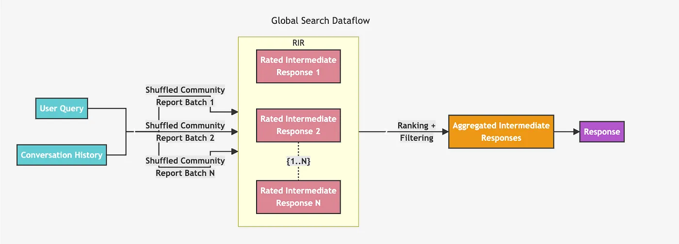
Global retriever architecture. Image from https://microsoft.github.io/graphrag/posts/query/0-global_search/
We have to decide which define in advance which hierarchical level we want to iterate over, which is a not a simple decision as we have no idea which one would work better. The higher up you go the hierarchical level, the larger the communities get, but there are fewer of them. This is the only information we have without inspecting summaries manually.
Other parameters allow us to ignore communities below a rank or weight threshold, which we won’t use here. We’ll implement the global retriever using LangChain as use the same map and reduce prompts as in the GraphRAG paper. Since the system prompts are very long, we will not include them here or the chain construction. However, all the code is available in the notebook.
def global_retriever(query: str, level: int, response_type: str = response_type) -> str:
    community_data = graph.query(
        """
    MATCH (c:__Community__)
    WHERE c.level = $level
    RETURN c.full_content AS output
    """,
        params={"level": level},
    )
    intermediate_results = []
    for community in tqdm(community_data, desc="Processing communities"):
        intermediate_response = map_chain.invoke(
            {"question": query, "context_data": community["output"]}
        )
        intermediate_results.append(intermediate_response)
    final_response = reduce_chain.invoke(
        {
            "report_data": intermediate_results,
            "question": query,
            "response_type": response_type,
        }
    )
    return final_response
Let’s now test it.
print(global_retriever("What is the story about?", 2))Results
The story primarily revolves around Ebenezer Scrooge, a miserly man who initially embodies a cynical outlook towards life and despises Christmas. His transformation begins when he is visited by the ghost of his deceased business partner, Jacob Marley, followed by the appearances of three spirits—representing Christmas Past, Present, and Yet to Come. These encounters prompt Scrooge to reflect on his life and the consequences of his actions, ultimately leading him to embrace the Christmas spirit and undergo significant personal growth [Data: Reports (32, 17, 99, 86, +more)].
### The Role of Jacob Marley and the Spirits
Jacob Marley’s ghost serves as a supernatural catalyst, warning Scrooge about the forthcoming visitations from the three spirits. Each spirit guides Scrooge through a journey of self-discovery, illustrating the impact of his choices and the importance of compassion. The spirits reveal to Scrooge how his actions have affected not only his own life but also the lives of others, particularly highlighting the themes of redemption and interconnectedness [Data: Reports (86, 17, 99, +more)].
### Scrooge’s Relationships and Transformation
Scrooge’s relationship with the Cratchit family, especially Bob Cratchit and his son Tiny Tim, is pivotal to his transformation. Through the visions presented by the spirits, Scrooge develops empathy, which inspires him to take tangible actions that improve the Cratchit family’s circumstances. The narrative emphasizes that individual actions can have a profound impact on society, as Scrooge’s newfound generosity fosters compassion and social responsibility within his community [Data: Reports (25, 158, 159, +more)].
### Themes of Redemption and Hope
Overall, the story is a timeless symbol of hope, underscoring themes such as empathy, introspection, and the potential for personal change. Scrooge’s journey from a lonely miser to a benevolent figure illustrates that it is never too late to change; small acts of kindness can lead to significant positive effects on individuals and the broader community [Data: Reports (32, 102, 126, 148, 158, 159, +more)].
In summary, the story encapsulates the transformative power of Christmas and the importance of human connections, making it a poignant narrative about redemption and the impact one individual can have on others during the holiday season.
The response is quite long and exhaustive as it fits a global retriever that iterates over all the communities on a specified level. You can test how the response changes if you change the community hierarchical level.
Summary
In this blog post we demonstrated how to integrate Microsoft’s GraphRAG into Neo4j and implement retrievers using LangChain and LlamaIndex. This should allows you to integrate GraphRAG with other retrievers or agents seamlessly. The local retriever combines vector similarity search with graph traversal, while the global retriever iterates over community summaries to generate comprehensive responses. This implementation showcases the power of combining structured knowledge graphs with language models for enhanced information retrieval and question answering. It’s important to note that there is room for customization and experimentation with such a knowledge graph, which we will look into in the next blog post.
As always, the code is available on GitHub.
Essential GraphRAG
Unlock the full potential of RAG with knowledge graphs. Get the definitive guide from Manning, free for a limited time.

Share Article


Explore
Related Articles

Getting Started With Neo4j Aura: A Guide to the Leading Cloud Graph Database
Building Stateful AI: Integrating Aura Agent Lifecycle with MCP and Persistent Memory