Mix and Batch: A Technique for Fast, Parallel Relationship Loading in Neo4j

Solutions Engineer, Neo4j
14 min read

If you’ve worked with Neo4j at scale — meaning you’ve wanted to load millions or billions of relationships — you have probably encountered this DeadlockDetectedException error message at one time or another:
org.neo4j.kernel.DeadlockDetectedException: ForsetiClient[transactionId=10128,
clientId=85] can’t acquire UpdateLock{owners=client: ForsetiClient…
This is the message you get when you try to write relationships to the same node at the same time when using a multi-threaded loading program.
I was recently working with Apache Spark using Databricks and ran into the deadlock error above. At the time of this post’s publication (June 2024), the Neo4j Connector for Apache Spark documentation page states:
“To avoid deadlocks, always use a single partition (with coalesce(1) or repartition(1)) before writing relationships to Neo4j.”
If I followed this advice, all the relationships I have would be loaded serially, which would prevent locking. However, it’s also much slower than I would prefer. I wanted my load to go faster, so I dug in a little more and rediscovered a technique that others before me used to parallelize their relationship loads.
The result is that I got my relationships to load two to three times faster.
Problem in a Nutshell
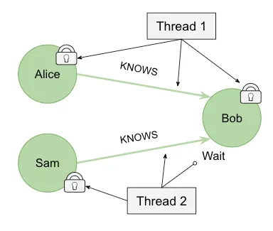
When Neo4j writes a relationship, it must lock the source and destination nodes. If more than one thread is trying to write to the same node at the same time, the second thread will need to wait until the lock frees up.
The diagram below illustrates this behavior. We want to write Alice KNOWS Bob and also Sam KNOWS Bob. In this case, Thread 1 grabs the lock on Alice and on Bob. Thread 2 grabs the lock on Sam but will have to wait for the lock on Bob to be freed before it can be written. In this simple case, the lock would be quickly freed so Thread 2 could write. But let’s add another thread and another relationship and see what happens.
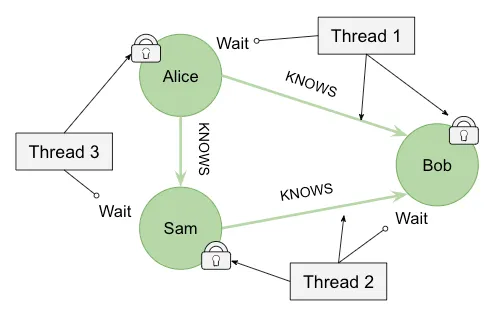
We also want to write that Alice KNOWS Sam, and we’ve added another thread for performance reasons. Now Thread 1 locks Bob, Thread 3 locks Alice before Thread 1 can get it, and Thread 2 locks Sam before Thread 3 can get it. Now we are in a deadlocked situation and the load fails.
When you load data at scale, these situations can occur quite frequently. Neo4j provides several mechanisms to handle deadlocks, such as deadlock retries. Neo4j has also added some product features, such as Relationship Chain Locks, but these haven’t completely eliminated the problem. The technique I will present in this post prevents threads from writing to the same nodes at the same time and, therefore, avoids the deadlock problem.
Mix and Batch Formula
The way to avoid deadlocks is to ensure that no two threads are accessing the same node at the same time. I’ve come up with this recipe that explains the steps to follow:
Prep
- Divide start node IDs and end node IDs into non-overlapping sets.
- Combine to make a partition code.
Mix
3. Lay out partition codes into a table.
4. Gather partition codes into batches — all partition codes must have unique column and row IDs per batch.
Batch
5. For each batch, use the partition code to partition the data — one partition per thread.
6. Load one batch at a time.
I’ll explain the steps using an example. Later, I’ll provide an example using Apache Spark.
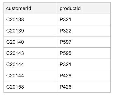
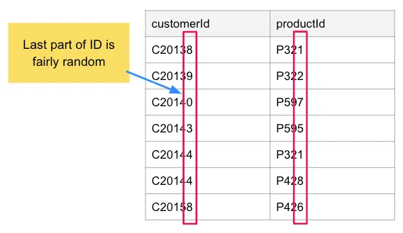
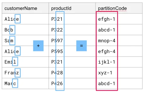
Imagine you have a set of customers that have bought some products. A sample of your dataset looks like this:
You want to write the BOUGHT relationship with the following Cypher:
MERGE (c:Customer {id: row.customerId})
MERGE (p:Product {id: row.productId})
MERGE (c)-[:BOUGHT]->(p)
We’ll follow the recipe to allow a large dataset like this to be imported in parallel.
Step 1: Divide Start and End Node IDs into Non-overlapping Sets
Note that the last part of the ID in our sample dataset is fairly random. In large datasets, the last digit should have a fairly even distribution. Given this, we can use the last digit of an ID to divide source nodes and end nodes into non-overlapping sets.
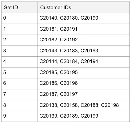
In this small dataset, we only have one customer set with more than one customer ID — the eighth set contains C20138 and C20158. However, you can imagine that as the dataset is extended, we could have something like this:
Each set will end up containing roughly 10 percent of the input data. We would also use the same technique for product. At this point, we don’t actually have to filter and split up the sets yet; we just need to know that when we pick part of the ID that it results in a fairly even distribution of IDs across the sets. It’s OK for some sets to have more than others — even a skew of 30 percent or more in one resulting set will result in faster load performance.
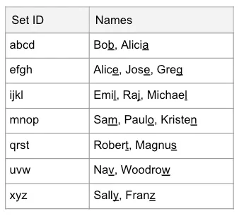
Using this particular dataset and using the last digit results in 10 sets for both customers and products. However, the Mix and Batch recipe doesn’t really care because it just needs the IDs divided up into non-overlapping sets. If you had a list of names as in our diagram before — Alice, Bob, and Sam — you could use the last letter and decide that names ending in a, b, c, or d are in set 1, those ending in e, f, g, or h are in set 2, etc. This scheme would result in seven sets (26/4).
An example of this scheme would be:
Step 2: Combine to Make a Partition Code
We need to combine our two set identifiers to make a partition code:
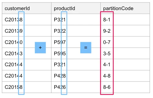
I am joining these as a string and adding this string value as another column. I am doing this because, from an implementation perspective, I can manipulate a DataFrame in Spark using this approach. If you were to implement this approach in a programming language, such as Java, it might be easier to keep them in memory as two-element arrays ([8,1], [9,2], [0,7], etc.).
One important thing to note is that the partition code comprises the set identifiers for each ID set. In our case, when we use the last digit, it just happens that the last digit is the set identifier. However, let’s imagine that our dataset has customerNames and productIds instead, and that productIds will be grouped into sets of 20 using the last two digits. Doing this, we may end up with something like this:
Here, productId has five sets:
- Set 0 contains productIds that end in 0–19.
- Set 1 contains productIds that end in 20–39.
- Set 2 contains productIds that end in 40–59.
- Set 3 contains productIds that end in 60–79.
- Set 4 contains productIds that end in 80–99.
We use the same sets (abcd, efgh, etc.) from the previous example. The rows with Bob and Marc end up with the same partition code, abcd-1, since the set IDs for customerName and productId are the same.
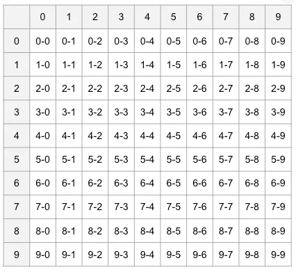
Step 3: Lay Out Partition Codes Into a Table
In this step, we take all possible set identifiers and place them in a grid. We’ll split the partition code to form the row and column IDs and place each partition code in the right spot. The following table shows the partition codes for our customerId productId dataset.
Using the partition codes for the customerName and productId with the two-digit groupings, we would end up with this for our square:
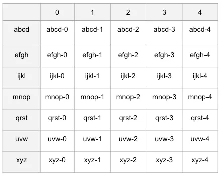
Now instead of a 10×10 grid, we have a 7×5 grid since there are seven rows and five columns.
Step 4: Gather Partition Codes Into Batches With Unique Column and Row IDs Per Batch
This is where the magic happens. To avoid deadlocks, we need to make sure that we aren’t processing cells 1–0 and 2–0 at the same time, for example. Why? Because we see the productId set 0 is present in both cells. If we are processing the same set of products at the same time, we have a much greater chance of a deadlock.
The same goes for 3–1 and 3–2; the cells both use orderId set 3 and can’t be processed at the same time because deadlocks could occur. So what do we do? We gather the cells like this:
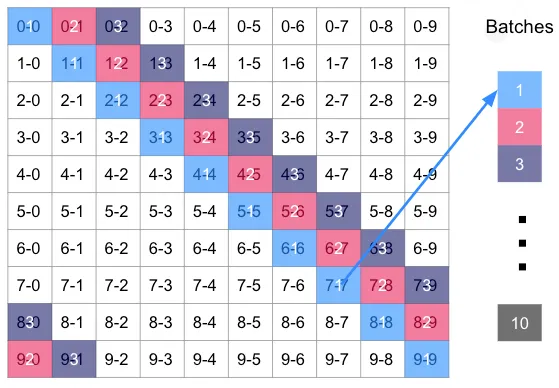
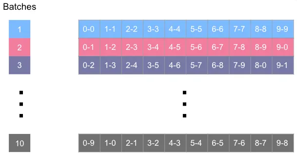
- Cells 0–0, 1–1, 2–2, 3–3 through 9–9 are all put into Batch 1
- Cells 0–1, 1–2, 2–3 through 8–9 and wrapping around to 9–0 go into Batch 2
- Cells 0–2, 1–3, 2–4, etc wrapping around to 8–0 and 9–1 go into Batch 3
We do this until we have 10 batches. Here, we moved left to right across the grid to form the batches. We would have gotten the same amount of batches and the same cells in each batch if we had moved from top to bottom because in this grid, the number of rows equals the number of columns. But what about the grid where they aren’t the same? Let’s look:
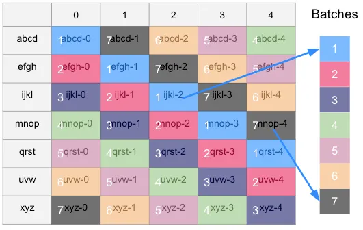
We get seven batches now. The number of batches will equal the larger of either the number of columns or number of rows. In this case, it was easier to move from top to bottom to get the batches, since the number of rows was greater than the number of columns.
Step 5: For Each Batch, Use the Partition Code to Partition the Data, One Per Thread
At this point, we have arranged our partition codes into batches, and for all partitions within each batch, there is no overlap between datasets. In the 10×10 grid case, our batches should look like this:
Within each batch, we now need to separate the data into different partitions by using the partition code. The number of partitions within a batch determines the number of threads we can use to load the data. The following diagram shows how each data partition can be assigned to a thread for processing.
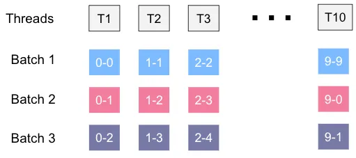
I’ve been using the term thread, but this actually may be a process, queue, or any other mechanism where you can split data up and have it processed in parallel.
Step 6: Load One Batch at a Time
Now that the data is partitioned, we execute the load. We need to process one batch at a time, and make sure that every partition within that batch is fully loaded before moving to the next batch.
You’ll note that when the data is very evenly distributed, most threads should finish at the same time within a batch. If we have a skewed distribution, some threads may finish and become idle while the larger partitions finish processing. This is OK — it may result in slightly slower loading overall, but will still be faster than loading all data with a single thread.
Apache Spark Example
In Apache Spark, data in one dataset can be spread out across different machines in the cluster to enable data processing in parallel. In the Neo4j case, this can result in deadlocking without our Mix and Batch techniques, so the guidance is to use repartition like so:
def writeTableToNeoSinglePartition (tableName, cypherQuery):
    df = spark.read.table(tableName).repartition(1)
    result = (df.write
        .format("org.neo4j.spark.DataSource")
        .option("url", url)
        .option("authentication.basic.username", username)
        .option("authentication.basic.password", password)
        .option("query", cypherQuery)
        .mode("Overwrite")
        .save()

writeTableToNeoSinglePartition("clicks", """
    MATCH(user:User {userId: event.userId})
    MATCH(news:News {newsId: event.newsId})
    MERGE(user)-[r:CLICKED]->(news)
    """)
The function writeTableToNeoSinglePartition accepts a tableName and a Cypher statement. In this case, our Cypher statement is creating relationships and will need to lock the user and news nodes every time the CLICKED relationship needs to be written. For a set of users with the same common interests, such as reading the same news articles, we have a high chance of deadlocks. Therefore, we follow the guidance in the docs and call:
df = spark.read.table(tableName).repartition(1)
This takes the data spread out over the cluster machines and puts it all on one machine, allowing it to be processed serially. Ultimately, we don’t want to process the data in a single thread, so we will implement the Mix and Batch technique.
Apache Spark Mix and Batch
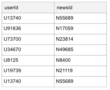
To implement Mix and Batch, we need to implement recipe steps 1–6 to make our load go faster. Let’s take a quick peek at our data, which has a similar format to our previous examples:
As a prerequisite, we’ll use some PySpark functions, so we need to import them:
from pyspark.sql.functions import col, substring, concat_ws
We’ll also load our data into a DataFrame (called df):
df = spark.read.table(tableName)
Steps
1. We can use the last digit of userId and the last digit of newsId to break apart the data into sets. We’ll use the substring function to accomplish this.
substring(df[‘userId’], -1, 1)
substring(df['newsId'], -1, 1)
This looks at the value in each cell, goes back one character, and takes one character. For U13740, this will be 0; for N55689, this will be 9, etc.
2. We use substring and concat_ws to form the partition code:
concat_ws(‘-’, substring(df[‘userId’], -1, 1), substring(df[‘newsId’], -1, 1))
We use the withColumn function to add the partitionCode value as an additional column called partitionCode, and we store this in a new DataFrame called newDf:
newDf = df.withColumn(‘partitionCode’, concat_ws(‘-’, substring(df[‘userId’], -1, 1), substring(df[‘newsId’], -1, 1)))
3 & 4. We define a getPartitionsAndBatches function to create our grid. This function assumes a square, so it won’t work in the 7×5 case we saw before, but it works for 6×6, 8×8, 10×10, etc. Since our set IDs are the digits 0–9 for both rows and columns, it will just loop through the numbers 0–9 in two nested loops. We calculate the value k as the first part of the partition code using the modulo operator (%):
# tableSize = 10 means a 10x10 table
def getPartitionsAndBatches (tableSize):
    batches = []
    for i in range(tableSize):
        partitions = []
        for j in range(tableSize):
            k = (i+j)%tableSize
            partitions.append(str(k) + '-' + str(j))
        batches.append(partitions)
    return batches
To give an example of how k is calculated, let’s assume a 3×3 square. We will cycle through 0–2 for i, and 0–2 for j. As we cycle through the numbers, we get:
i = 0, j = 0, k = 0
i = 0, j = 1, k = 1
i = 0, j = 2, k = 2

i = 1, j = 0, k = 1
i = 1, j = 1, k = 2
i = 1, j = 2, k = 0  // 1+2 = 3, modulo 3 = 0, therefore k = 0

i = 2, j = 0, k = 2
i = 2, j = 1, k = 0  // 2+1 = 3, modulo 3 = 0, therefore k = 0
i = 2, j = 2, k = 1  // 2+2 = 4, modulo 3 = 1, therefore k = 1
The result is a set of batches containing diagonal cells. You can see this when we run it with tableSize 3:
print(getPartitionsAndBatches(3))
It produces:
[[‘0–0’, ‘1–1’, ‘2–2’], [‘1–0’, ‘2–1’, ‘0–2’], [‘2–0’, ‘0–1’, ‘1–2’]]
This shows the partition codes arranged in batches. The first batch has partition codes 0–0, 1–1, and 2–2. For our case, we want to run it with a value of 10, so we’ll do that and store the value in the batches variable.
batches = getPartitionsAndBatches(10)
5. We need to split the data by partitionCode in each batch. To do that, we’ll define a small filterByPartitionCode helper function, which will accept a larger dataset and return a filtered dataset that matches any values passed in the partitionSet, which are all of the partitionCode values for a batch:
def filterByPartitionCode(df, partitionCol, partitionSet):
    return df.filter(col(partitionCol).isin(partitionSet))
We call that function to create a new DataFrame, batchDf, for each batch. The variable batchDf only contains the data for that batch. Then, we use the repartition function and specify the value 10 and the partitionCol name, which will split our data by the partitionCode value across 10 different partitions. For the first batch, this means data for partitionCode 0–0 would be on partition 1, partitionCode 1–1 on partition 2, partitionCode 2–2 on partition 3, etc.
    batchDf = filterByPartitionCode(df, partitionCol, partitionSet)
    parallelRelDf = batchDf.repartition(10, partitionCol)
6. We put everything together and execute the load, executing steps 1–5 during processing, loading one batch at a time.
We’ll need another helper function, writeDfToNeo, that accepts a DataFrame and writes it directly to Neo4j using the provided cypherQuery:
def writeDfToNeo(df, cypherQuery):
    result = (df.write
        .format("org.neo4j.spark.DataSource")
        .option("url", url)
        .option("authentication.basic.username", username)
        .option("authentication.basic.password", password)
        .option("query", cypherQuery)
        .mode("Overwrite")
        .save()
Now we define the function that does all the work, writeRelTableToNeo, which accepts a tableName, startNodeCol, endNodeCol, and a cypherQuery:
def writeRelTableToNeo(tableName, startNodeCol, endNodeCol, cypherQuery):
    df = spark.read.table(tableName)
    partitionCol = 'partitionCode'
    # Steps 1 and 2
    newDf = df.withColumn(partitionCol, concat_ws('-', substring(df[startNodeCol], -1, 1), substring(df[endNodeCol], -1, 1)))
    # Create separate DataFrames for each batch
    # Steps 3 and 4 previously created the variable 'batches'
    # Step 6 - the for loop runs each batch is sequence
    for index, partitionSet in enumerate(batches):
        # Step 5 is done by the next 2 lines
        batchDf = filterByPartitionCode(newDf, partitionCol, partitionSet)
        parallelRelDf = batchDf.repartition(10, partitionCol)
        writeDfToNeo(parallelRelDf, cypherQuery)
The function has comments where each step is executed. All of the partition codes within a batch are assigned to the partitionSet variable, and each batch is executed successfully in the for loop. The data for the batch is filtered and stored in batchDf and split by partition code into parallelDf. Finally, we use the writeDfToNeo helper function to execute the load. Since we partitioned the data across multiple cluster members, Apache Spark executes the partitions for the batch in parallel.
Here is an example of calling writeRelTableToNeo:
writeRelTableToNeo("clicks", "userId", "newsId", """
    MATCH(user:User {userId: event.userId})
    MATCH(news:News {newsId: event.newsId})
    MERGE(user)-[r:CLICKED]->(news)
    """)
We load the clicks table, specify the userId and newsId as the start and end cols, and pass in the Cypher statement to load the relationships.
Results
I tested this approach by loading data from Databricks into a Neo4j AuraDS environment. I ran multiple data loads with different datasets, and the results are shown below.
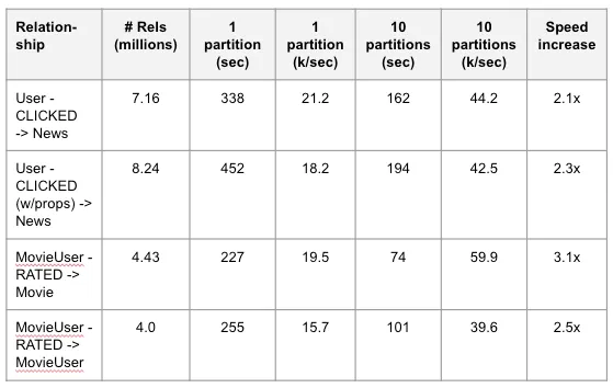
Using the Mix and Batch technique, I was able to make the load go two to three times faster. The maximum speed I got was around 60,000 (60k) relationships per/sec. I provisioned my Databricks environment and AuraDS environment to have at least 12 vCPUs each, so I was hoping for even faster performance, but I’m still pleased with my results. Many factors influence write speed: disk IOPS, network latency, and many other factors within the Neo4j database itself, so the speed increase doesn’t correspond linearly with the number of threads.
However, 2–3 times faster can really be a game-changer. Here is a table showing the time benefits:
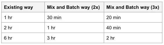
We can see that load time could be cut by up to one-third of its original time.
The more I got into Mix and Batch and began experimenting with parallel loading and attempts to speed up relationship loading, more avenues of exploration opened up. I don’t have time to elaborate in detail here, but here are a few additional things I started exploring:
- When I filtered datasets on a different thread before the partitioning, I got a 5–8% speed-up in time.
- When I loaded non-exclusive relationship sets at the same time (User-CLICKED->News, and MovieUser-RATED->Movie), I further sped up the load.
- Ten partitions/batches worked best, but 8 and 15 also worked well.
- By using more digits than just one to create the partition code, you can smooth out the distribution of the cells.
- This technique could be applied to streaming data, but it requires more investigation and experimentation.
Some sample code can be found here: https://github.com/Neo4jSolutions/parallel-relationships, which contains a few Python notebooks. The Full demo.ipynb is the most mature, with some of the others being early experiments.
If you need to load large volumes of relationships into Neo4j, I hope you’ll give this technique a try.
References
- J. Porter and A. Ontman, “Importing Relationships into a Running Graph Database Using Parallel Processing”, https://arxiv.org/pdf/2005.04093
- Neo4j Connector for Apache Spark, https://neo4j.com/docs/spark/current/
Mix and Batch — A Technique for Fast, Parallel Relationship Loading in Neo4j was originally published in Neo4j Developer Blog on Medium, where people are continuing the conversation by highlighting and responding to this story.
Share Article


Explore
Related Articles

Finding the Fastest Way Out: How Dijkstra’s Algorithm Finds Shortest Paths