Graph Databases Explained: How Relationships Change Everything

Head of Developer Organic Marketing, Neo4j AuraDB
31 min read


Cover image: Main hall of the East Building of the National Gallery of Art, Washington, DC. [Public domain.]
In this chapter:
- The most important fact: Neo4j graph models correspond with how you think about data
- Watch how the relational data model replaces real-world relationships with predicate logic relationships
- See how biomedical researchers built a Parkinson’s Disease research model with Neo4j instead of RDBMS, keeping all real-world relationships intact
- Find out how and why Neo4j eliminates JOINs, yet at the same time, expedites queries
- Build a Neo4j graph model for yourself using existing, simple data
Here is the most important thing you’ll ever need to know about Neo4j graph databases, right up front: Graph methodology is intentionally designed to resemble as closely as possible the conceptual model of information that you would convey to other people, if you were to draw it on a whiteboard. The way you would visualize data in your mind, forms the foundation of the graph database. And if you have a database that isn’t yet a graph database, once you’ve built a conceptual model for it, most of your schematic work is done.
If you begin with that in mind, your path to results will be short.
A modern database is a service. It carries out instructions from an application, and the means of communication is the driver. Neo4j does not change these facts. But because a Neo4j database is well-informed as to what the final results of a report or a query should actually contain, what does change are the instructions that an application communicates to the database via the driver. You no longer have to task the application with instructing the database as to how to assemble, step-by-step, intermediate tables of interim results, which you would then have to stitch together as best you could, to produce the table from which you siphon off a set of final results.
Granted, there are certifications for the type of job skills required for a data engineer to manage and execute these tasks. With Neo4j, you no longer need them. How that changes the way you work, and the way your organization and business work, may be up to you.
Where your work process changes, and why
You may be wondering, what’s the tradeoff? Where is the bargain one has to make to attain these much promised, and perhaps grandiosely hyped, results? Here it is: If you’re using existing data in tables, spreadsheets, or key/value stores, you do need to import that data into Neo4j. In the import process, you literally draw the relationships using circles and arrows. That’s the graph part. You can do this with the symbols you use in Neo4j’s Cypher language, or you can choose instead to do this with your mouse, or even your stylus on a tablet. Neo4j enables you to model the data your application will use to solve problems, using a graphical representation that very closely approximates how you’d draw the composition of that data on a whiteboard. With this model, you embed the relationships into the data from the start.
There’s work involved. It comes at the beginning of the database creation process. This work will save you days, perhaps years, of time expended during the information gathering process. Then it will save you more time in the processing of that information. Big queries on huge data sets consume marginally longer stretches of time for graph data than for relational data.
You may have read somewhere that Neo4j is a fancy, graph-shaped container for an overblown data silo. That’s false. If you use ours or anyone’s native graph database system, and you wind up with a data model that is not connected, not networked, and does not account for all the possible relationships between all the elements of data in your entire data warehouse, you’re doing it wrong. When you do graph right, with the right graph, you will not see even the semblance of where data silo walls would have been in a relational environment or an unprocessed data lake. In fact, to be honest, you’re much more likely to become confused by the abundance of connections and relationships, than the lack of them.
In Summary, So Far
Neo4j is a system that enables you to build the connections and relationships that you know already exist in your data, into your database from the beginning. There’s extra up-front effort involved with this, but it’s handled in a sensible, intelligible, intuitive, and perhaps even enjoyable way. The payoff comes with the greatly enhanced value of the results you receive. They’re more informational, more analytically relevant, and especially in the case of large and huge data sets, faster.
Using a Graph Without Knowing It

An all-hands meeting at Proof Technologies in Austin, Texas. [Photo licensed by Unsplash.]
The best way to demonstrate these assertions is with examples of projects that are actually happening in the real world.
Perhaps you’re familiar with this: In the field of small business economics, a lucrative concept called the entrepreneurial ecosystem (sometimes “entrepreneurship ecosystem”) has been taking shape. At its core is the idea that there is, or at least can be, a self-sustaining environment of economic innovation that benefits small and emerging businesses, when the communities they serve actively work to foster their development.
The keyword there is “community.” Rather than tackle the problem of growing new businesses wholly on a national scale, this ecosystem theory suggests that innovation happens first and foremost on a local level — perhaps at the scale of cities, but maybe scaling down further to counties or townships. In the US, the Small Business Innovation Research Program (SBIR) is betting that a methodology may exist for connecting large-scale business-nurturing facilities and institutions, such as government programs issuing federal grants, with several smaller-scale, more local-level facilities and “accelerators,” including universities and venture capital firms.

Figure 1.1. A conceptual framework for an entrepreneurial ecosystem, proposed by researchers at The University of North Carolina at Chapel Hill, Cal Poly Pomona, the University of Oregon Lundquist College of Business, and Wake Forest University School of Business.
Figure 1.1 depicts the perceived relationships between the various components of a functional entrepreneurial ecosystem, as envisioned by four university researchers on the subject. Except for the trivial fact that these researchers are using boxes rather than circles or ellipses, and that the properties of relationships are color-coded, what they’ve produced is a legitimate graph model. There are clear relationships between the entities, and each relationship has one of three possible types. It doesn’t take a college course for a person such as yourself to gather how this network of entities enables cooperation.

Figure 1.2. The Entrepreneurial Ecosystem model as a Neo4j graph database model.
Translating this model into the form and format of a Neo4j database graph, such as the one depicted in Figure 1.2, will perhaps take the novice less than a half-hour, and a skilled practitioner even less time. This is not an artist’s rendering of what a graph model would look like if we had the resources to visualize it properly; this is the actual graph model produced by Neo4j.
Here, the items that were grouped together into boxes in the conceptual framework, are broken out into individual nodes. Each node may have a type, denoted as encircled labels separate from their names. Each node also has a property, which fulfills the function of the color-coding in the original model’s legend. Nodes are associated with each other by arrows, which represent relationships. Each arrow only has one pointer, so a two-headed arrow in the conceptual model is replaced here by two arrows pointing opposite directions. Each relationship has a type that explains what a subject node does to, or for, an object node. You’ve just experienced the basics of graph modeling.
While we were converting the conceptual model into a Neo4j graph, the tool we used automatically generated a CREATE statement in the Cypher language. This statement can be executed within Neo4j to produce the actual database where all this information would be collectively stored. Unlike most any other computer language you might use for any purpose, Cypher is a bit pictorial with its syntax:
CREATE (:Resource)<-[:Collaborates with]-(Government:Organization)-[:Collaborates with]->(`Entrepreneur firm`:Organization)-[:Innovates]->(:Resource),

(:Resource)<-[:Collaborates with]-(Government)-[:Collaborates with]->(:Resource),

(:Resource)<-[:Innovates]-(`Entrepreneur firm`)-[:Innovates]->(:Resource),

(Government)<-[:Innovates]-(`Entrepreneur firm`)<-[:Provides capital to]-(Government)<-[:Collaborates with]-(`Entrepreneur firm`)-[:Collaborates with]->(`Small firm`:Organization)-[:Produces]->(:Resource),

(:Resource)<-[:Produces]-(`Research institution`:Organization)-[:Collaborates with]->(`Entrepreneur firm`)<-[:Collaborates with]-(Accelerator:Organization)<-[:Collaborates with]-(`Entrepreneur firm`)-[:Collaborates with]->(`Large firm`:Organization)-[:Produces]->(:Resource),

(`Small firm`)-[:Collaborates with]->(`Entrepreneur firm`)-[:Collaborates with]->(`Research institution`)-[:Produces]->(:Resource),

(:Resource)<-[:Produces]-(`Small firm`)-[:Produces]->(:Resource),

(:Resource)<-[:Produces]-(`Large firm`)-[:Produces]->(:Resource),

(`Large firm`)-[:Collaborates with]->(`Entrepreneur firm`),

(`Research institution`)-[:Produces]->(:Resource),

(:Resource)<-[:Produces]-(Accelerator)-[:Produces]->(:Resource)
At first, it may seem a Cypher statement such as this relatively long one, wouldn’t be too easy to read. But look more closely, and you’ll see something astonishing you won’t find in any other computer language: A Cypher CREATE statement contains all the components of a graph, expressed using a syntax that leverages special characters such as parentheses, square brackets , and even –[arrows sticking through brackets]-> to replace circles, label boxes, and arrows. It disconnects all the elements of a graph, then lays them end-to-end in sequence.
The ecosystem researchers might have used this graph modeling method to produce a framework for their APPRISE platform scheme. They did not. They opted instead for a traditional, relational approach. While that approach shows all signs of being functional, the research team actively demonstrates what they characterize as their system’s viability, by way of its complexity. Here in Figure 1.3, for example, is one real example produced by the APPRISE team of just one leaf of the schematic their system uses to map interrelationships between data sourced from multiple entities:

Figure 1.3. Part of the primary and foreign key structure
Data sourced from 14 separate small business organizations, especially from JSON documents (two examples of which, with formal entity identifiers GRID and ORCID, appear on the right of Figure 1.3), contain unique identification codes that serve as keys. GRID (Global Research Identifier Database) refers to a database of research and educational organizations, while ORCID (Open Researcher and Contributor ID) is a registry of research organizations maintained by a non-profit project. The integer field FIPS_CODE refers to a common code that US Government agencies use to identify United States counties. The minimal area in which an entrepreneurial ecosystem may inhabit, in the APPRISE scheme, is a county.
With a bit of effort, though not too much, you can deduce the purpose of a schema such as this one. The two tables that jointly record every federal grant and loan made, to whom, and under which contract, are SAM and USASpending. These are publicly available, heterogenous data sets, for anyone who has the time or bandwidth to download them. What links these two tables together in the APPRISE schema are their shared DUNS_CODE fields, which are unique identifiers generated by Dun & Bradstreet for recognized business entities. Data pertaining to each grant appears in the USASpending table; data recording to whom it was made appears in SAM. Technically, the sharing of these keys between tables constitutes what relational databases consider to be relationships.
Notice, however, they’re not the same relationships as in the original conceptual model. Here is where you come to realize the dichotomy of a relational database schema: It maintains separation between tables for the sake of data integrity, but then rewires relationships between those tables for the sake of informational value. This process is what we refer to as normalization, referring to the phrase “normal form” made relevant at IBM by E. F. Codd, who first brought relational logic to common use.
It’s a process presented to the world at large as the easiest way to go about managing records from multiple sources. “Each separate data source,” the APPRISE researchers wrote for their report, “results in a table, or entity, that relates to another entity through a primary key, or unique identifier, that matches a foreign key in the connected table. This relational structure allows for easy retrieval and storage of large amounts of information across many sources.”
The two principal tables at issue here — SAM and USASpending — will always be separate files. In this case, they were designed for PostgreSQL. No database schema can alter that fact. For PostgreSQL or any relational database, the act of assembling a set of records as fundamental or as ordinary as showing who received what when, will always require JOIN operations, and perhaps also UNION operations as well. Such statements often end up being expressed within long and extensive scripts of SQL instructions. Altering the structure of the tables, were anyone to decide to do so, would undoubtedly alter these scripts. And because nobody wants to have to alter the scripts, everyone avoids altering the structure of the tables.
If you want to see the substance with which institutional silos are constructed, here it is.
This is the first issue that a native graph database such as Neo4j resolves. It is perhaps the first and foremost reason why an organization may want to use it: With a graph, the conceptual model of data is the operational model of data. You don’t have to take multiple steps of abstraction and disassembly, arriving at “normalized forms” of your data that your database engine can recognize as unique and integral, just so you can reassemble all those forms together into an entity that’s useful for a practical purpose.
In Summary, So Far
The typical schema of a relational database devolves from the original relationship model that people conceive in their minds and draw on whiteboards. This is intentional and deliberate, done for the sake of the data. “Normalization” ensures the continuity and integrity of data that requires unique records, so that indexing and relational logic can work.
The Right Graph from the Beginning

Genomic sequencing chips used by the National Cancer Institute’s Division of Cancer Epidemiology and Genetics.
[Photo licensed by Unsplash.]
To see this assertion put into practice, let’s change subject domains from macro-economics to biomedicine. The fact that standard data table structures are subject to change when new discoveries or new ways of interpretation come to fruition, is something biomedical researchers saw coming perhaps before macro-economists did.
In 2021, three researchers in the AI department at Universidad Nacional de Educación a Distancia in Madrid published an article in the Oxford University journal Database asserting the degree to which native graph databases, including Neo4j most prominently, have outmoded relational databases in complex clinical research. “The relational paradigm,” they wrote, “is very appropriate for well-defined data structures that are unlikely to change and translate naturally to tables, and the relations among its entities are not numerous and not as relevant as the entities’ attributes.”
But when the layout of the data schema has to be broken out into something as complex as Third Normal Form (3NF), as was the case with the APPRISE model, they continued:
… this layout would require referencing (joining and sub-querying) several tables multiple times, potentially with various filters, ultimately eroding the query’s performance. Also, complicated queries may end up being rather cumbersome. Thus, designing a relational model for highly interconnected data poses an engineering challenge, especially when the model requires fine-grained semantics, which involves a trade-off between implementing specialized relations (more tables) or limiting the expressiveness at the expense of semantics.
The Common Fund of the US National Institutes of Health has supported two projects for cataloguing scientifically observed biomedical phenomena. One is the Library of Networked Cell-based Signatures (LINCS), which is an effort to record every perceivable way that human-body cells respond to negative influences, or perturbations — including chemical reactions, genetic disorders, neurodegenerative disorders, heart disease, even “micro-environments.” Anything capable of generating a negative influence on a human cell is catalogued by LINCS as a perturbagen. The other is the Illuminating the Druggable Genome Project (IDG, no relation to the publisher), whose database is the product of extensive data mining through the world’s biomedical literature, for data on chemical and pharmaceutical agents, and their biological targets in the human body.
Here are two heterogenous data sets (see if this rings a bit familiar to you now) produced by two projects whose aims run parallel to each other. To bring these data sets together, a team of researchers led by the Indiana University School of Informatics, Computing and Engineering developed what they call a Knowledge Graph Analytics Platform (KGAP).
For their project, it would appear that the KGAP team actively avoided the relational approach. One member of the IU team had previous experience with implementing relational models, including the University of New Mexico’s CARLSBAD [PDF], described as “A Confederated Database of Biochemical Activities.” It’s a relational amalgam from five main data sources, brought together using what the New Mexico team described as “separate extract, transform and load (ETL) pipelines. . . for each of the data sources.” The IU team was blunt in characterizing CARLSBAD as “limited in analytics performance and versatility by its implementation as a relational database.”
KGAP utilizes a logic schematic that maps the relationships between data elements found in both LINKS and IDG data sets, presented here as Figure 1.4.

Figure 1.4.The basic data model for the Knowledge Graph Analytics Platform (KGAP), produced by the IU Schools of Informatics, Computing and Engineering, in conjunction with Data2Discovery, Inc.
Once again, it’s not exactly a Neo4j graph, but you can imagine it might not take long to produce one. This time, that’s exactly what the team did. One part of that Neo4j graph, depicting the same relationships shown above in a manner that translates directly to a Cypher statement, appears in Figure 1.5:

Figure 1.5. One basic LINCS/IDG relationship concept re-styled as a Neo4j graph.
The KGAP project does not do away with ETL. Extracting, transforming, and loading data from separate sources into Neo4j, is still a thing you have to do. It just doesn’t require some ridiculous metaphorical paradigm adoption to bring it about. In fact, if anything, it’s mundane.
So here’s an example of what the IU team accomplished: Suppose you’d like to know the relative likelihoods of all the known drugs in the world, to have some positive impact (or negative) on the specific genes whose known mutations are associated with Parkinson’s Disease. That’s the nervous system disorder responsible for ceaseless tremors, and gradual loss of motor control.
Every drug that’s been discussed in biomedical research literature has a context of information associated with it, represented in the graph in Figure 1.5 above as Concept. Meanwhile, known perturbagens may be identifiable by the effects that these same known drugs have on them, positive or negative. That identification comes up as a Signature. Human cell types are also identifiable by the same Signature. That pairing enables a graph database to extract and identify the relationships with each Gene with which cells may be associated.
From these relationships, evidence may be extracted that chains drugs to genes. The researcher may then look backwards into which concepts led to drug discoveries and experiments, to determine whether or how similar treatment regimens can be applied to identifiable genetic disorders, such as those related to Parkinson’s.
Here, in its entirety, is the actual Cypher query used by the IU team to generate final scores, or z-scores, that indicate the relative ranking of relationships between catalogued drugs and genetic symptoms:
MATCH p=(d:drug)-[]-(s:signature)-[r]-(g:Gene), p1=(s)-[]-(c:Cell)

WHERE (d.pubchem_cid in [2130, 2381, 4167, 4601, 4850, 4919, 5095, 5572, 6005, 6047, 23497, 26757, 30843, 31101, 47811, 59227, 77991, 119570, 1201549, 3052776, 4659569, 5281081, 10071196, 135565903])

WITH g, sum(r.zscore)/sqrt(count(r)) AS score

RETURN g.id, g.name, score

ORDER BY score DESC
It’s not SQL, and there’s no SELECT statement. Instead, Cypher’s MATCH statement is drawing a pattern, and there’s blanks in that pattern. The relationship types between the empty brackets [] are unknown. The type we want to know more about here is r. If you have the graph in Figure 1.5 in front of you, you can compare its pattern against the one drawn by the MATCH statement itself.
From there, the rest of the instruction looks quite a bit more like SQL. The WHERE clause makes perfect sense for those who know about looking up multiple property values. The embedded functions sum() and sqrt() are familiar, and the assignment of their result to the variable score is direct and obvious. So without a huge instruction manual or nineteen hours of hands-on video, you can probably see how Cypher would become not only familiar but comfortable to any experienced data engineer who has worked with SQL.
However, there remains one huge difference that any SQL expert would point out in a heartbeat: This entire query was conducted with a single instruction, consuming only five lines of code. A chain of third-order relationships of this magnitude, for any general-purpose SQL database, would require sequences of JOIN statements, and perhaps UNION statements, that would at best have consumed a small booklet.
How big this is
Let’s be clear about the magnitude of this, because we run the risk of actually understating it: Programs capable of processing relationships at this scale, have been running for decades. And in a way, that’s the problem. Overcoming the exponential time losses associated with processing chained relationships with relational databases, has typically required supercomputers. Even then, runtimes have consumed months, rather than hours. With Neo4j, you no longer require a supercomputer. Just a cloud server will do.
What’s more: The methodologies involved with Neo4j at this scale, technically do not qualify as artificial intelligence. There’s no neural network at work here. We’re not using fake neurons or axons, weights or pulleys, or any form of convolutional logic. Neo4j isn’t as basic as predicate logic, but it’s not a backpropagated neural network. The complexity level is somewhere in-between. Because of this, results are not bound or restricted by probabilistic logic. With neural networks, your results always come paired with confidence levels, whose values are always less than 100%. With Neo4j, your confidence in your results is whole and complete.
In Summary, So Far
Building a Neo4j graph model from a natural, realistic model of relationships, bypasses the steps involved with normalizing, de-normalizing, and re-normalizing data. Yet the result is a more robust database format, along with a more capable platform, that lets researchers, engineers, economists, and other higher-order scientists continue to think the way they think. If that describes you, then you can be not only a Neo4j user but a Neo4j data engineer, rather than look to hire someone who “speaks data” to run or manage the database for you.
Build Your First Graph Relationship

[Photo by Kvalifik, licensed by Unsplash]
Now, let’s give you the opportunity to see exactly how you can model the basic class of relationship we’ve discussed here thus far, with the Neo4j AuraDB platform. What follows is an exercise you can do right now, without having to purchase anything, and without having to convert or translate some massive data set. Instead, we’ll use a public data set with which you may already be familiar: the Northwind retail database, which is a fictitious model of a very basic retail operation, originally created by Microsoft to demonstrate database principles with Access and SQL Server.
Although Neo4j hosts already imported databases that replicate the Northwind data set, for this exercise, we’d like to take you through the process of importing its CSV table files. This way, we can approximate (on a smaller scale) the general steps that the IU researchers would take to import their knowledge graph and drug indications data sets, and build relationships around them. Download the CSV files yourself from Neo4j’s GitHub location.
Next, follow the instructions below to create an instance of AuraDB Free, populate it with our test data using the Data Importer, and create your first relationships graph:
Initiating the AuraDB Free Database Instance
- Near the top of the Neo4j AuraDB presentation page, click Start Free. AuraDB will display the sign-in panel shown in Figure 1.6.

Figure 1.6. Registering your AuraDB Free account.
- Enter your Email address and Password (or click Continue with Google to leverage your existing Google login). Then click Login. If this is your first login to AuraDB, you will see the Instances screen shown in Figure 1.7.

Figure 1.7. The Instances screen, which should be mostly blank after your first login.
- Click New Instance. AuraDB will present you with a panel of choices, shown in Figure 1.8.

Figure 1.8. The Create an instance setup panel.
- By default, AuraDB Free is pre-chosen. In the Instance Name text box, enter a new database server name, such as “NWTest01.”
- Under Starting dataset, choose Empty database.
- Click Create Instance. In a moment, AuraDB will show the credentials panel shown in Figure 1.9.

Figure 1.9. The credentials panel will be the only place for receiving the pre-generated password, and will only be shown once.
- To store a local copy of this automatically generated password, click Download, then in your file manager or finder window, choose a suitable location and save your file. The password will contain random characters and will appear to be encrypted, but is actually raw text; however, nothing that will take place with this sample database will include sensitive information. Soon, the Instances screen will show one instance NWTest01. In a few moments, the instance will be fully generated, and will enable commands as shown in Figure 1.10.

Figure 1.10. A new instance is created.
- To begin the data import process, click Import. You’ll be asked to log onto your new database instance for the first time, with the panel shown in Figure 1.11.

Figure 1.11. The main AuraDB database login panel.
NOTE: Be sure to take note of the Connection URL that appears in the database login panel. As you log in again later, this field may appear blank, and you’ll need that address to fill in your database’s deployment location.
- Once you’ve logged in successfully, the Data Importer screen will appear, showing you an empty mapping area, as shown in Figure 1.12.

Figure 1.12. The Data Importer screen, where your first relationship graphs will be drawn.
NOTE: After several hours of inactivity, AuraDB will automatically pause any active databases operating in the Free tier. If you log into AuraDB later and find your instance has been paused, in the Instances screen, click Resume Database (the right arrow in the lower right corner of the instance frame) to un-pause it. The resumption process may take a minute or so longer than was required to initiate the instance.
For this example, we only require the files orders.csv, order_details.csv, products.csv, and suppliers.csv. From your file manager or finder window, drag these four files into the Drag & Drop zone of the Data Importer screen. The Files pane will respond by showing the column names for each imported table, along with sample contents from the first record of each table.

Figure 1.13. The relational schema for Microsoft’s first permutation of the Northwind sample database.
If you’ve worked with relational data to any degree, then the relational schema in Figure 1.13 will either be immediately familiar to you, or at least instantly interpretable. Each principal table utilizes a unique, usually automatically generated, primary key. Microsoft Access labeled these fields with gold key icons. You can easily see where relationships are formed between foreign keys in some tables, and their identically named primary key counterparts in other tables. There isn’t anything particularly difficult about this schema — at least, not conceptually.
Notice in this schema a table called Order Details. It’s a secondary table with no primary key of its own. Rather, it’s an element in a “third-order” relationship — one that picks up the pieces from two detached relationships from Orders and Products. Its purpose is to record a product item that has been ordered by someone, and relate that item to a specified purchase order. This data was separated into its own table as part of the act of normalization, which ensures the uniqueness and integrity of records in a relational database.
You would not want to record the details for each purchase order, in the same record. If a purchase order contained 16 items, you’d be replicating the freight and shipping region data 16 times. However, when you need to construct an SQL query that calculates the shipping costs for an order with 16 items in it, you actually do have to generate a JOIN table. In that table, in memory, that shipping data does become replicated. You have a huge table, but at least it’s not stored that way.
With a relational database, every mildly complex interrelationship has to be resolved by reconstructing data tables into forms you wouldn’t dare use for storage, just so a query can extract the right information iteratively. It’s a method that seemed efficient enough, at least back when PC clones were limited to 640K of addressable RAM, and 720K double-sided diskettes were sold as technological marvels that dwarfed 360K single-sided diskettes. Simply put, there wasn’t storage space for us to construct stronger data models up-front, that would let you avoid the whole normalization/de-normalization route.
So what you will do in the following exercise (if you’re not paying close attention, you might not know you’re even doing it) is reconstruct this Northwind data model in a graph form where the separation of details from core identifiers is no longer required.
How to draw a graph node
Your first Neo4j AuraDB node, at the center of several critical relationships, will be Product, which will serve as the counterpart for the Products table in the relational schema. In the schema above, you’ll see that as a table, it’s intended to have relationships with Order Details and Suppliers.
For AuraDB to comprehend relationships, you need to draw the symbols that represent them as part of the graph. Here’s how to put Product at the center of your graph:
- In the upper left corner of the graphing area, click Add node. A circle immediately appears in the center. (If a helper cue comes up marked Sketch your graph, read it, take note of its animation, and click on Got it.)
- Type any key to make the cursor appear in the center of the new node (or click on the node).
- Type Product. (You don’t need to hit Enter.)
- To create the node to which Product relates, click and hold the blue circle around Product, then drag that circle in any direction. An arrow will automatically be created pointing from Product to the new node.
- Release the mouse button, type any key to make the cursor appear in the new node, and type Order. Your screen should resemble Figure 1.14.

Figure 1.14. The first pair of nodes, and the primordial relationship between them.
How to graph a relationship
With a graph database, relationships are not implied through identical key names, but rather expressed as part of the graph structure —as an arrow between two nodes. So when a CSV file or TSV file has a primary key field as a column for its records, the existence of that field does not have to be removed for the graph. Instead, you let Data Importer know which imported fields were the primary keys, and which ones were the foreign keys that referred to them. You saw those relationships back in Figure 1.3, where arrows pointed from foreign key locations in tables, to primary locations in others. Fields from the related tables become properties of the graphed nodes.
For the specific relationship we just created, it’s actually pointing the wrong way. An order may include a reference to a product, so we want to change the direction of the arrow. Then we want to give that relationship (or what graph practitioners would call the “edge”) a name, to denote the substance of the relationship. It’s this qualitative substance that a relational schema cannot represent without the creation of an entirely new table, including two foreign keys that would bond both other tables (a “third-order relation”). For a graph, you need not concoct such a table; what you do instead is this:
- Click the relationship arrow.
- In the upper left corner of the Mapping Details pane, click the bi-directional arrow icon (which may resemble two staples squashed together). The arrow will change directions.
- Click on the Type field, and to give the relationship a name, type Includes. This word will be inscribed next to the arrow.
- To bind the Product node to the products.csv file, click the Product node, then in the Mapping Details pane, under File, select csv. Repeat this same process to bind Order to the orders.csv file.
- To bring fields into the Product node as properties, click the Product node, then under Mapping Details, click on Select from file. In the Select from file pane that pops up, click Select all.
- Click Confirm. In the left pane, the names of mapped fields that are now properties, will be given green spots. In the right pane, under the Properties tab, the same mapped names will be listed, along with their ascertained types.
NOTE: Neo4j does not represent dates and times as exclusive data types. Instead, they are imported and utilized as text strings.
- To identify the field being used as the identifier (primary key) for the Product node, click that node (if it isn’t already selected), then in the Mapping Details pane, under ID (lower right), click the Please select a property combo box and choose productID. Note that the dotted line around the node becomes solid at this point.
- Repeat this process from step 5 to bring fields into the Order node as properties, this time choosing orderID as the identifier.
- Next, to begin specifying how orders relate to products, click the Includes relationship arrow.
- In the Mapping Details pane, under File, choose order‑details.csv.
- Under From, select orderID.
- Under To, select productID. Note that the dotted line for the arrow becomes solid at this point.
- Under the Properties tab, click Select from file. In the pane that pops up, click unitPrice, quantity, and discount. These are fields that will be used to qualify the relationship. Click Confirm.
At this point, one of the most critical relationships from Northwind — one that had been implemented as a separate “third-order relation” table in the RDBMS — has just been modeled. You now have eliminated the need for hundreds, perhaps thousands, of JOINs. Next, you’re about to repeat that feat for the other side of the relationship. To specify the supplier relationship, do the following:
- Using the same method you used earlier to produce the Order node relating to Product, drag a new node in any direction from Product and name it Supplier. Notice in Figure 1.15 below, if you want your graph to look prettier, as you’re holding the mouse button down, you may see a red dotted circle as you try to place this new node. This is not a warning indicator, or anything having to do with the structure of the underlying database; it’s just to snap your new node into place if you want it to orbit your main node from an equidistant altitude, if you will.

Figure 1.15. The red dotted line helps you snap your next new node into position.
- In the Mapping Details pane, under File, choose csv.
- Under the Properties tab, click Select from file. In the popup, click Select all, then click Confirm.
- Under ID, select supplierID. The node circle will change from dotted to solid.
- Select the new relationship arrow, reverse its direction, and name it Provides.
- Under File, choose csv.
- Under From, choose supplierID.
- Under To, choose productID. Your graph model should now generally resemble Figure 1.16.

Figure 1.16. The completed third-order relationship modeled in Neo4j Data Importer.
Once this process is complete, AuraDB has everything it needs to generate a database from these nodes, in the Neo4j format. You do this by clicking on Run Import. Momentarily, Data Importer will show you tables of results like the ones in Figure 1.17.

Figure 1.17. Data import results from the Northwind data set.
The series of steps you’ve just followed substitutes for the nothing that you would need to do for beginning a query process with a relational database. Neo4j’s competitors argue that implementing a graph database creates steps that would not be required for an RDBMS. You’ve just seen what those steps are. Not so scary now, are they?
As a result of the input graph you’ve created, Neo4j generates an output graph, representing the actual relationships between each record in the imported tables. Figure 1.18 shows what an output graph for this small segment of an arguably small database, looks like from maximum altitude. These nodes represent real records from the three main Northwind tables we utilized, qualified by that fourth table that had served only to represent relationships in the older model.

Figure 1.18. The output graph from imported data in the Northwind orders, products, and suppliers tables.
Ending Our Subservience to Relational Logic
The whole point of a database management system is to be able to query and extract records that group together elements of related data. Since the 1960s, the prevailing wisdom has dictated that relationships be boiled down to pure predicate logic. That’s the easiest form of logic that can be directly translated into the opcodes and operands of binary-encoded procedures.
None of these facts have somehow shifted sides from right to wrong. But processors are literally thousands of orders of magnitude more powerful now, and memory no longer has to be carted around on cylinders loaded with dollies onto lorries. Human beings do not have to translate their ways of thinking into mathematical formulas, of the variety that drips from the bottom corners of blackboards in university auditoriums, simply for them to ascertain a list of drugs that might have a chance of treating genetic disorders. There’s room in the computer now to make the process work more like the way we work naturally.
If we hadn’t been so concerned with maintaining continuity and backwards compatibility as virtues or selling points, we might have all been working this way thirty years ago already. Hurricanes might have damaged less property and fewer lives. Pharmaceuticals and innovative treatments might have brightened the livelihoods of thousands more people. And indeed, if we may be this bold, certain pandemics might never have happened.
Back to the whiteboard
At its core, a graph database is an information store whose model is visual by design. That’s on purpose. Seeing what you’re modeling enables you to model it more easily and more efficiently. Neo4j calls this a “whiteboard-friendly” approach to data modeling.
You might think this is what fundamentally distinguishes a graph database from any other category. You know the relational model, in which most of the world’s data that makes any sense, is stored. You’ve seen enough — perhaps too many — unstructured data stores, where most of the world’s other data is maintained, presumably for future processing.
Frankly, what truly distinguishes graph databases are something even more important: A graph database relies upon the model, rather than the index, to locate data. Put another way, the graph database processor finds what it’s looking for by traversing the model that’s already there, rather than referencing an index that had to be generated in advance, or compiling a view or a join that wasn’t there before.
The graph data model is a map. It depicts relationships between data entities not as outputs from queries, but inputs to the model. You define data by depicting its relationships to other data. This way, when you solve a problem that involves finding relationships, the graph database engine does not have deduce those relationships. They’re already in the database, so they’re simply recalled from storage.

Figure 1.19: A simple graph depicting relationships between three data entities, in the context of Twitter users who belong to each other’s social network.
Figure 1.19 above depicts another input to a graph database, in much the style as you produced yourself earlier, but with a few more types of details. With conventional relational database operations, the information depicted here would be an output. You would have a table of individual people, all of whom would have complete names, but also unique identifying numbers that the end user would never see. The relationships depicted by FOLLOWS –> would be compiled into a separate, second-order table, where the identifiers for the follower and the followed entity would be paired together. Finding the people who are followed by folks who are themselves followed, would require producing even more tables in memory that are joined composites formed from replicated chunks of the second-order table.
You could equip a relational database with the graphical tools it would need to produce a graph like Figure 1, as an output — a solution to a complex operation triggered by a simple query. And because that query, and queries like it, are indeed so simple, the maker of that database would market it as “easy to use.” Sure, for you, maybe.
But “use” doesn’t stop with retrieving stored data. If you’re an applications engineer, you’re leveraging that data to solve problems. And if you’re a database engineer, your job is to ensure not only the availability of the database behind solving those problems, but also scaling the database and the operations around it, as the amount of stored data increases — as databases are typically wont to do.
With a graph such as Figure 1.19 in place, you don’t need another map just to find data that matches a parameter, fits a pattern, or solves a problem. So about two-thirds of the work you’ve had to do just to deduce or derive a result that yields a practical solution to a real-world work problem, is no longer necessary.
Why haven’t we been using data like this all this time?
Never in the history of any technology, anywhere — baking bread, brewing beer, broadcasting television — has an outmoded method immediately disappeared from common use. We continue to cope with the media we already know how to use. Familiarity is often a more valued commodity than efficiency.
This is especially true with data, whose format is a direct product of the processors and methodologies that produce and manage it. Not only are its processes already in place, but teaching how to use those processes requires a measure of stability and permanence that, in and of itself, perpetuates methods and substantiates talents. A relational database engineer would be immediately rendered a relic of a bygone era, were we to unanimously decide always to update our methods to match the moment. Every point release would spark a revolution.
So the global graph database revolution has not happened yet. This does not mean you can’t embrace the moment, today.
In Summary
What makes any database functional are relationships. With a relational database, relationships are implied from the data structure, then deduced by reassembling that structure for the purposes of specific queries. With Neo4j, relationships are built into the structure. No reassembly is required. This construction process requires extra effort during the database creation procedure, or during the import procedure. It’s not much extra effort, however, and it can be executed using an interactive, graphical procedure that’s fluid, intuitive, and sensible.
Where from here?
- What Is a Graph?
- Why Graph Technology Is the Future
- Why Connected Data Matters
- The Basics of Data Modeling
- Data Modeling Pitfalls to Avoid
- Why a Database Query Language Matters
- Imperative vs. Declarative Query Languages: What’s the Difference?
- Graph Theory & Predictive Modeling
- Graph Search Algorithm Basics
- Why We Need NoSQL Databases
- ACID vs. BASE Explained
- A Tour of Aggregate Stores
- Other Graph Data Technologies
- Native vs. Non-Native Graph Technology
Share Article


Explore
Related Articles

Mastering Fraud Detection With Temporal Graph Modeling


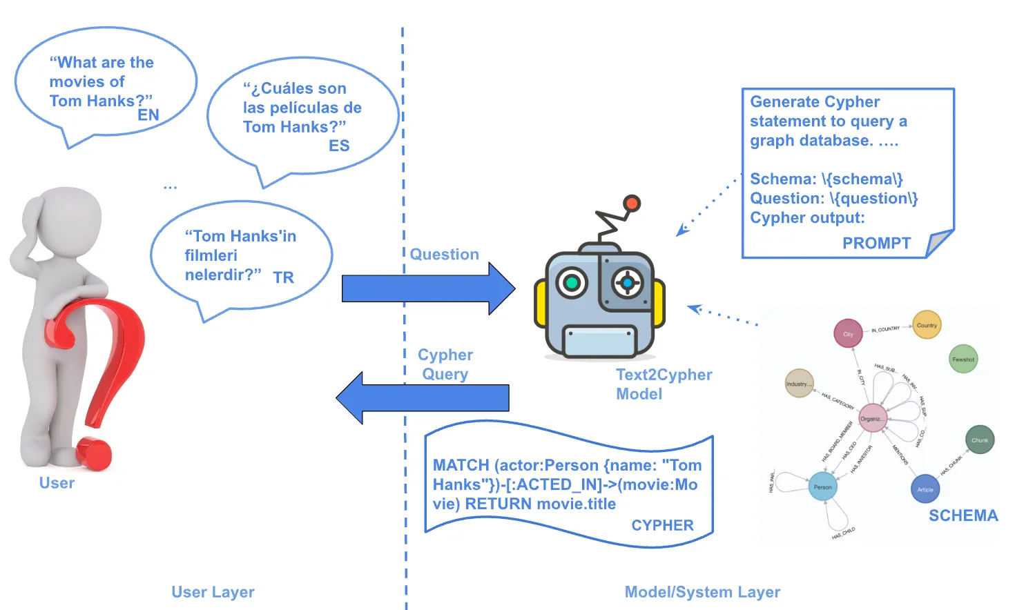
Text2Cypher Across Languages: Evaluating Foundational Models Beyond English