Build a Routing Web App With Neo4j, OpenStreetMap, and Leaflet.js

Hands-On Workshop Exploring Working With Road Network Data and Routing With Graph Algorithms

Running path-finding algorithms on large datasets is a use case that graph databases are particularly well suited for. While often pathfinding algorithms are used for finding routes using geospatial data, pathfinding is not just about geospatial data — we often use pathfinding graph algorithms with non-spatial data. We could be exploring neural pathways on a graph of the human brain, finding paths connecting different drug-gene interactions, or finding the shortest path connecting two concepts in a knowledge graph.

In this tutorial, we will see how to build a routing web application using the Neo4j graph database, data from OpenStreetMap and OpenAddresses, and Leaflet.js for rendering our web map. This post is adapted from a live online workshop I facilitated as part of Neo4j’s free online workshops that cover a variety of topics around building applications and analyzing data with graphs. You can find the video version of this workshop on the Neo4j YouTube channel.

To follow along with the workshop and complete the exercises you’ll need a free Neo4j AuraDB instance and a Python development environment, either locally or via a cloud programming environment like GitHub Codespaces.

Neo4j Aura: Your Free Graph Database in the Cloud

Neo4j Aura is Neo4j’s managed database service. We’ll first create a free Neo4j AuraDB instance. Be sure to download the connection credentials when creating your Neo4j instance — we’ll need that information later to connect to our database instance.

Working With OpenStreetMap Data in Neo4j

One of the main concepts I wanted to focus on in this workshop is how to work with OpenStreetMap data in a graph database like Neo4j. We’ll cover that but first, let’s explore OpenStreetMap a bit.

What Is OpenStreetMap?

OpenStreetMap (or OSM) is an amazing public open dataset of mapping and geospatial data covering the globe — all contributed by the community. OpenStreetMap contains information about points of interest, roads, walking trails, bike paths, and much more. OpenStreetMap is often used to power some of the largest and most popular map software.

The OpenStreetMap data model consists of nodes, ways, tags, and relations and is optimized for editing and maintaining a crowd-sourced dataset. The OSM data model is actually a graph that connects these core elements (nodes, ways, tags, and relations).

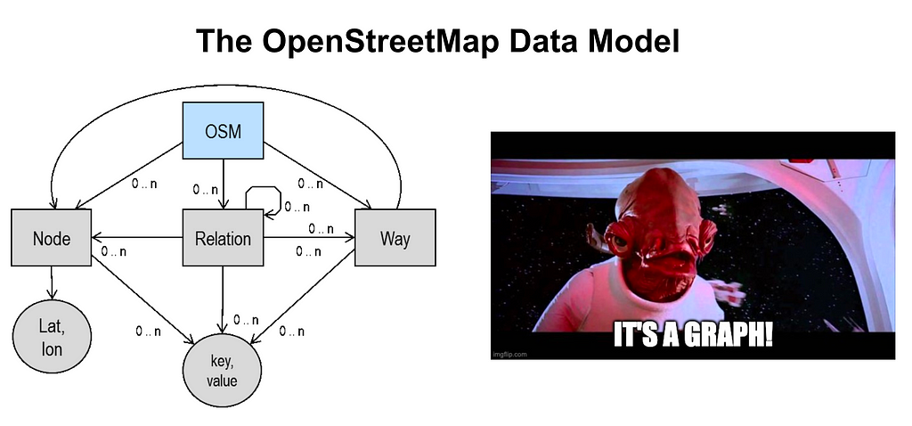
• Nodes — point features, for example, points of interest or part of a more complex geometry
• Ways — line features that connect nodes. Roads, buildings, parks, etc.
• Tags — arbitrary key-value pair attribute data describing a feature. Can be used on nodes, ways, and relations.
• Relations — organize multiple ways (or nodes) into a larger entity. For example, multiple road segments that make up a bus route. This is also how multipolygon geometries are represented in OpenStreetMap.

Two good resources for learning more about the OpenStreetMap data model are the Elements entry in the OSM Wiki and this page from MapBox.

Working With OpenStreetMap in Neo4j

We already said that the OpenStreetMap data model is a graph so what does working with OpenStreetMap data in a graph database enable us to do? There are many use cases for working with geospatial data in a graph database like Neo4j, but routing is a common geospatial graph problem. We can also apply graph data science to geospatial data when working with geospatial data as a graph (commonly called geospatial knowledge graphs).

Graph data science is the use of graph algorithms and graph data visualization techniques to make sense of data. Spatial graph data science is the application of graph algorithms to spatial knowledge graphs. OpenStreetMap provides a rich graph-based dataset that can be analyzed using graph data science.

For example, we could analyze a city’s road network using the betweenness centrality algorithm to identify important intersections and the Louvain community detection to identify neighborhoods. Visualization allows us to explore and interpret the results of these graph algorithms, facilitating an important part of our analysis.

Other spatial graph data use cases are more “transactional” or “operational” such as powering a web or mobile application. One example of this type of application is a travel guide application called Central Perk that we built as part of the Neo4j Livestream series using OpenStreetMap, Neo4j, React, Gatsby.js, and GraphQL. With this application, we enhanced the OpenStreetMap data graph with data from Wikipedia, crowd-sourced street-level images from Mapillary, routing, and point-of-interest search.

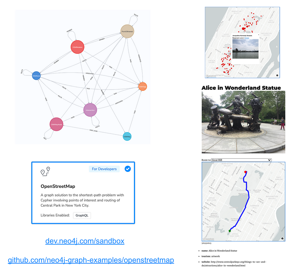
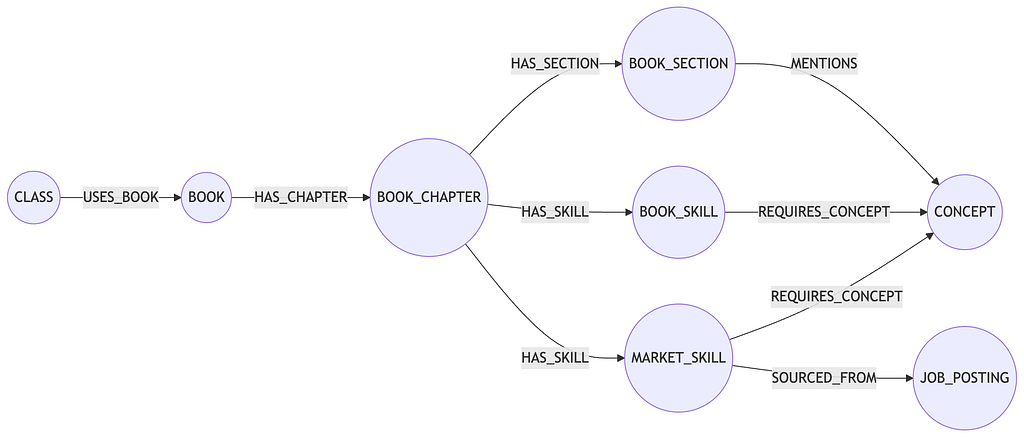
As you can see in the image above the property graph data model used to represent our OpenStreetMap data of Central Park maps directly to the data model used by OpenStreetMap: we are modeling OSM nodes, ways, relations, and tags as nodes in the graph. While this data model is optimized for maintaining and editing this large crowd-sourced dataset, it is not always the best data model for every application. Later we’ll see how to simplify this data model for our routing application.

There are several ways to access OpenStreetMap data, such as downloading the entire planet dataset or a subset in the OSM XML format which can then be converted to other formats or imported into databases. Another option is to query the OpenStreetMap Overpass API. The Overpass API enables programmatic access to subsets of OpenStreetMap data and powers tools like the QuickOSM QGIS plug-in for adding OpenStreetMap data to QGIS projects and the OSMNx Python package which enables working with road networks in Python created from data from OSM.

We’ll use OSMNx to build a routing graph in Neo4j that consists of a city road network.

The OSMNx Python Package

The OSMNx Python package was created at the Urban Planning lab at the University of Southern California for the purpose of analyzing road networks.

One powerful feature of OSMNx is the ability to simplify the network topology of the road network. As we saw above the OSM data model is a rich dataset optimized for editing that includes much additional information that might not be needed for working only with road networks, or for our purposes of building a simple routing application. For example, instead of keeping track of every point in a road segment as an explicit node in our data, are we only interested in intersections — nodes that connect two or more road segments.

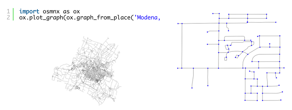
For our purposes of building a simple routing application this is a perfect fit.

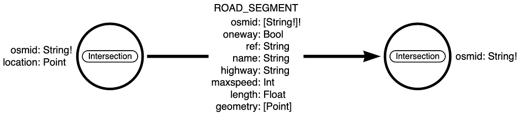
Importing OpenStreetMap Data Into Neo4j With OSMNx

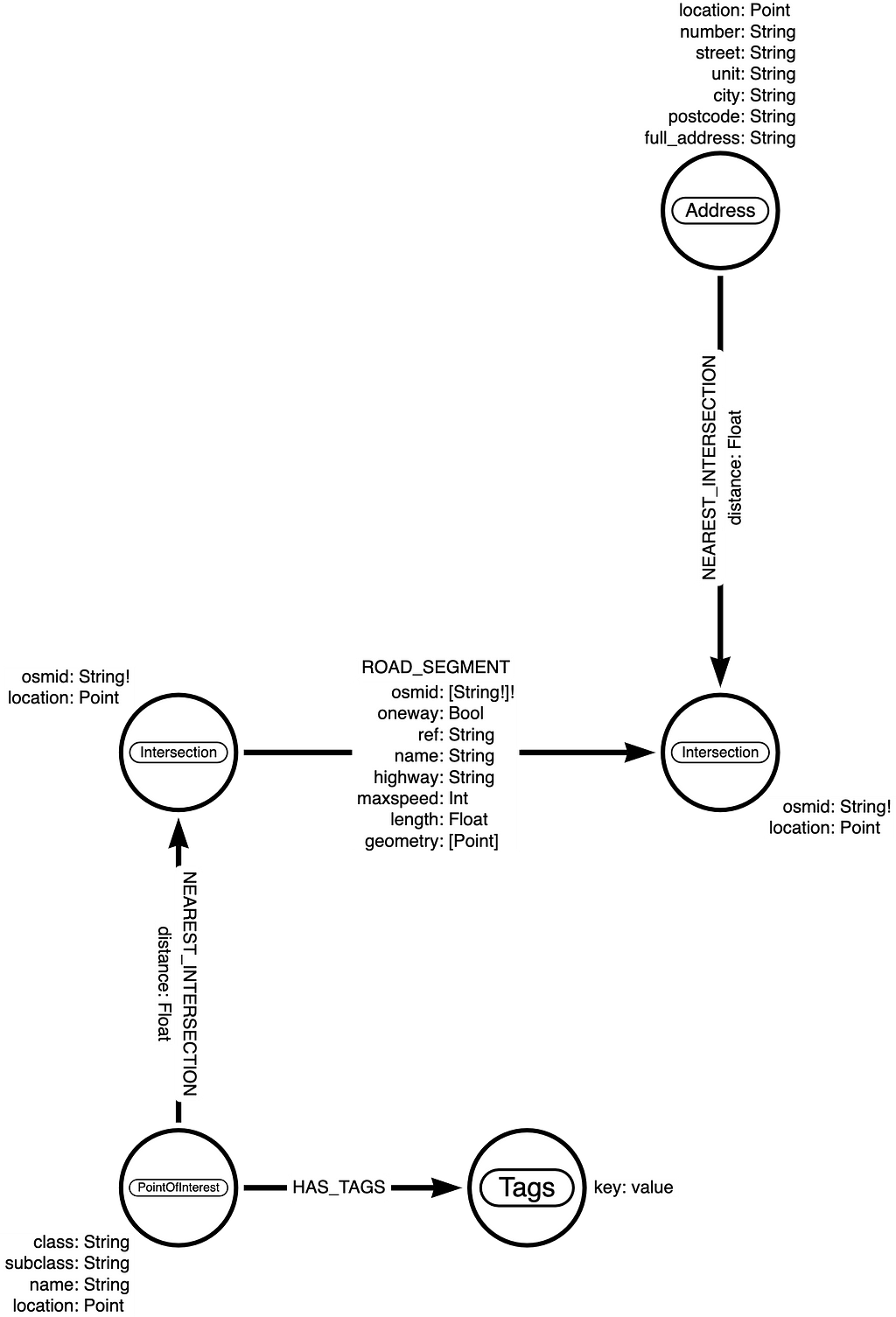
The first step of any data import project is to consider the data model to be used. In this case, we will model road intersections as nodes in the graph and road segments connecting intersections as relationships. We’ll use the osmid value to identify node uniqueness and we’ll store the latitude/longitude location of the intersection as Point type node property called location. We will store relevant information about the road segment as relationship properties, such as oneway, name, maxspeed, and length.

Let’s get started! We’ll install the OSMNx and Neo4j Python Driver packages:

pip install neo4j osmnx

Next, let’s make sure we can connect to our new Neo4j AuraDB instance using the Neo4j Python driver. Later, we’ll use the Neo4j Python driver to import data into Neo4j from OSMNx, but for now we’ll just run a simple Cypher query to see how to use the Python driver:

import neo4j


NEO4J_URI = "<YOUR_NEO4J_URI_HERE>"
NEO4J_USER = "neo4j"
NEO4J_PASSWORD = "<YOUR_NEO4J_PASSWORD_HERE>"

driver = neo4j.GraphDatabase.driver(NEO4J_URI, auth=(NEO4J_USER, NEO4J_PASSWORD))

CYPHER_QUERY = """
MATCH (n) RETURN COUNT(n) AS node_count
"""

def get_node_count(tx):
    results = tx.run(CYPHER_QUERY)
    df = results.to_df()
    return df


with driver.session() as session:
    df = session.execute_read(get_node_count)

df

#   node_count
#   __________
# 0  0

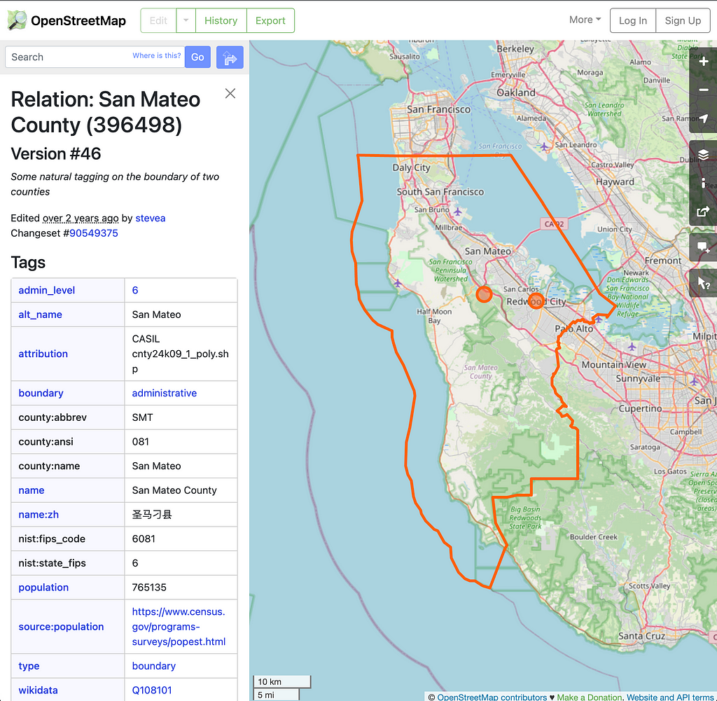
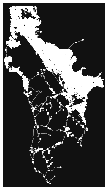
Now that we can connect to our Neo4j AuraDB instance, let’s see how to fetch OpenStreetMap data via OSMNx and import it into Neo4j. Let’s fetch the road network for San Mateo County.

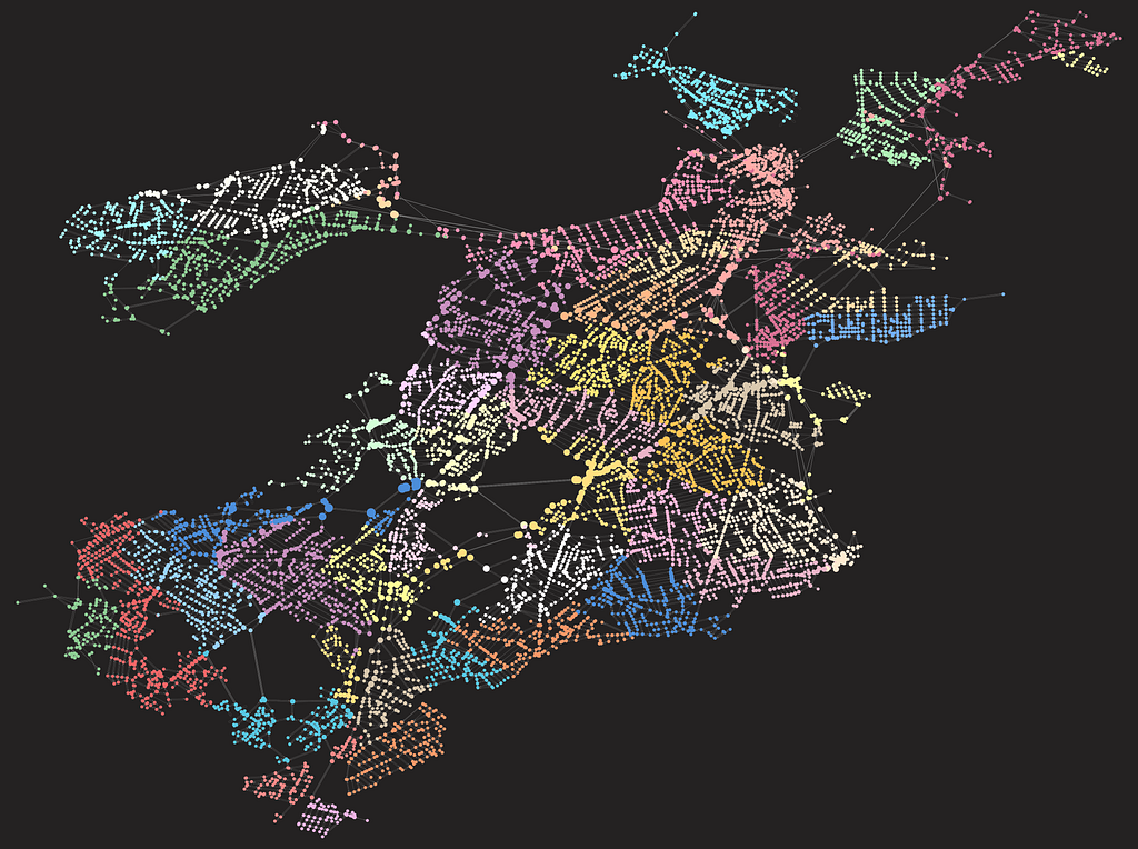
G = ox.graph_from_place("San Mateo, CA, USA", network_type="drive")
fig, ax = ox.plot_graph(G)

We can represent our road network as two GeoDataFrames, one for the nodes (intersections) and one for the relationships (road segments). A GeoDataFrame is an extension to a Pandas DataFrame but adds additional functionality for geospatial operations.

# Our road network graph can be represented as two GeoDataFrames

gdf_nodes, gdf_relationships = ox.graph_to_gdfs(G)
gdf_nodes.reset_index(inplace=True)
gdf_relationships.reset_index(inplace=True)

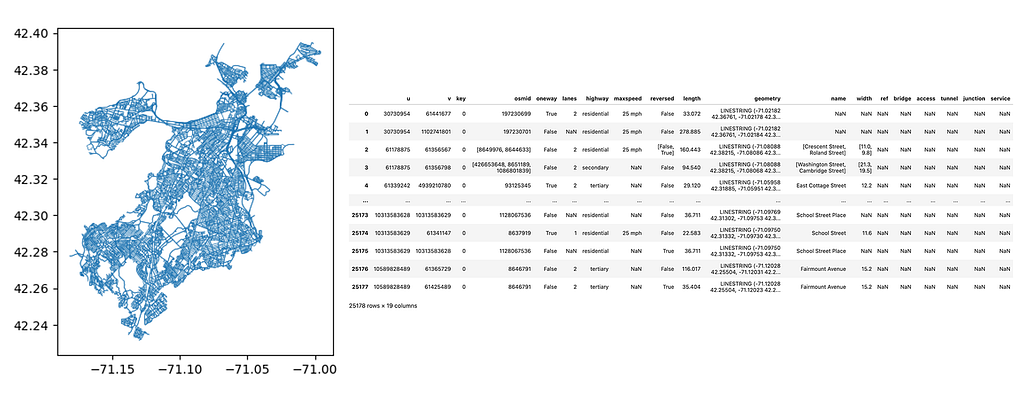
Now we have two GeoDataFrames gdf_nodes and gdf_relationships . Note that each GeoDataFrame has a geometry column that defines the geometry of the feature (each row is a feature).

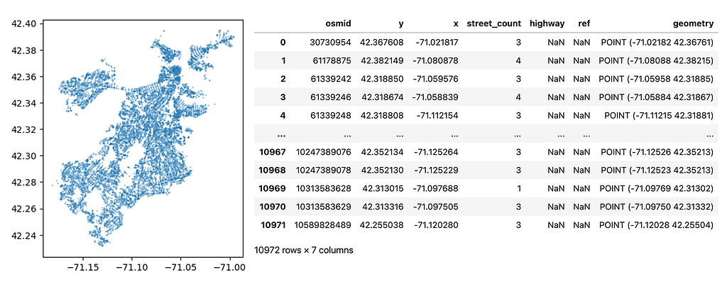
Our nodes have a point geometry, while the relationships are a linestring geometry, representing the road segment connecting two intersections.

To import these two GeoDataFrames into Neo4j we will first define a Cypher query that contains the logic for how to create data in the database, assuming a chunk of rows from the GeoDataFrame is passed as a parameter. This batching will allow us to import very large dataframes across multiple transactions in the database, making more efficient use of memory.

# First, define Cypher queries to create constraints and indexes

constraint_query = "CREATE CONSTRAINT IF NOT EXISTS FOR (i:Intersection) REQUIRE i.osmid IS UNIQUE"

rel_index_query = "CREATE INDEX IF NOT EXISTS FOR ()-[r:ROAD_SEGMENT]-() ON r.osmids"

address_constraint_query = "CREATE CONSTRAINT IF NOT EXISTS FOR (a:Address) REQUIRE a.id IS UNIQUE"

point_index_query = "CREATE POINT INDEX IF NOT EXISTS FOR (i:Intersection) ON i.location"

# Cypher query to import our road network nodes GeoDataFrame

node_query = '''
    UNWIND $rows AS row
    WITH row WHERE row.osmid IS NOT NULL
    MERGE (i:Intersection {osmid: row.osmid})
        SET i.location = 
         point({latitude: row.y, longitude: row.x }),
            i.ref = row.ref,
            i.highway = row.highway,
            i.street_count = toInteger(row.street_count)
    RETURN COUNT(*) as total
    '''

# Cypher query to import our road network relationships GeoDataFrame

rels_query = '''
    UNWIND $rows AS road
    MATCH (u:Intersection {osmid: road.u})
    MATCH (v:Intersection {osmid: road.v})
    MERGE (u)-[r:ROAD_SEGMENT {osmid: road.osmid}]->(v)
        SET r.oneway = road.oneway,
            r.lanes = road.lanes,
            r.ref = road.ref,
            r.name = road.name,
            r.highway = road.highway,
            r.max_speed = road.maxspeed,
            r.length = toFloat(road.length)
    RETURN COUNT(*) AS total
    '''

Then we create a function to use the Neo4j Python driver that chunks the rows of our dataframe into batches and executes our import Cypher queries, passing the rows from the dataframe for each batch.

# Function to batch our GeoDataFrames

def insert_data(tx, query, rows, batch_size=10000):
    total = 0
    batch = 0
    
    while batch * batch_size < len(rows):
        results = tx.run(query, parameters = {'rows': rows[batch*batch_size:(batch+1)*batch_size].to_dict('records')}).data()
        print(results)
        total += results[0]['total']
        batch += 1

And finally, create a session object and execute our data import:

# Run our constraints queries and nodes GeoDataFrame import

with driver.session() as session:
    session.execute_write(create_constraints)
    session.execute_write(insert_data, node_query, gdf_nodes)

# Run our relationships GeoDataFrame import

with driver.session() as session:
    session.execute_write(insert_data, rels_query, gdf_relationships)

Note that while our dataset for San Mateo county is quite small (18k nodes and 46k relationships) and we could have loaded both GeoDataFrames in a single operation, using this pattern will help us scale up when we need to import millions of rows.

Adding Addresses From Open Addresses

We now have a road network for San Mateo County stored in our Neo4j AuraDB instance. We could run our routing algorithms now to find intersection-to-intersection routing, but that’s not quite useful for our purposes as we want users to be able to route between points of interest or route between addresses.

OpenStreetMap does contain some address data, but another option for adding address data is OpenAddresses which compiles data on addresses around the world.

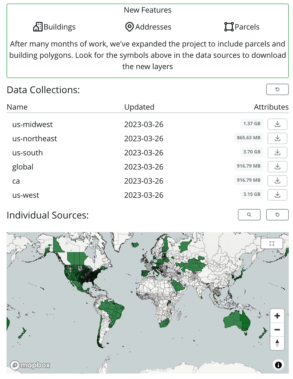
I downloaded the GeoJSON export of San Mateo country addresses from OpenAddresses. It looks like this:

{
  "type":"Feature",
  "properties":
    {
      "hash":"a98a4da3fa36d965",
      "number":"599",
      "street":"SKYLINE BLVD",
      "unit":"",
      "city":"DALY CITY",
      "district":"",
      "region":"",
      "postcode":" ",
      "id":"002011020"
    },
  "geometry":
    { "type":"Point",
      "coordinates":[-122.4995656,37.7033098]
    }
}

Let’s add our address data to our San Mateo County road network in Neo4j. We’ll add a node for each address, storing the address information and point location as a Point property on the node. Then we’ll find the closest intersection node in the graph and connect our Address node to it, storing the distance as a relationship property.

We also want to do something similar with points of interest. I’ve added it here to the data model, but we’ll leave this part as an exercise for the reader 🙂 As an example of how this might be possible see this blog post.

We can import GeoJSON in Neo4j using the apoc.load.json procedure.

CALL apoc.load.json("https://cdn.neo4jlabs.com/data/addresses/san_mateo.geojson") YIELD value
RETURN COUNT(value) AS num
// num: 286665

We can see that there are 287k features in this address GeoJSON dataset. We can use Cypher to create a node with the label Address for each feature. We’ll use the CALL {} IN TRANSACTIONS subquery to batch these 287k features across multiple transactions to more efficiently use memory.

:auto
CALL apoc.load.json("https://cdn.neo4jlabs.com/data/addresses/san_mateo.geojson") YIELD value
CALL {
  WITH value
  CREATE (a:Address)
  SET a.location = 
    point(
      {
        latitude: value.geometry.coordinates[1], 
        longitude: value.geometry.coordinates[0]
      }),
    a.full_address = value.properties.number + " " + 
                     value.properties.street + " " + 
                     value.properties.city + ", CA " + 
                     value.properties.postcode
SET a += value.properties
} IN TRANSACTIONS OF 10000 ROWS

Next, we will connect our Address nodes to our road network graph by finding the closest intersection node for each address and creating a CLOSEST_INTERSECTION relationship connecting the Address and Intersection nodes. For a given address, this Cypher query will find the closest intersection (using a subquery) and create a CLOSEST_INTERSECTION relationship:

MATCH (a:Address) WITH a LIMIT 1
CALL {
 WITH a
  MATCH (i:Intersection)
  USING INDEX i:Intersection(location)
  WHERE point.distance(i.location, a.location) < 200

  WITH i
  ORDER BY point.distance(p.location, a.location) ASC 
  LIMIT 1
  RETURN i
} WITH a, i
MERGE(a)-[r:NEAREST_INTERSECTION]->(i)
SET r.length = point.distance(a.location, i.location)

To batch this operation across multiple transactions to more efficiently use transaction state memory we will wrap this statement in a call to apoc.periodic.iterate:

CALL apoc.periodic.iterate(
  'MATCH (p:Address) WHERE NOT EXISTS ((p)-[:NEAREST_INTERSECTION]->(:Intersection)) RETURN p',
  'CALL {
  WITH p
  MATCH (i:Intersection)
  USING INDEX i:Intersection(location)
  WHERE point.distance(i.location, p.location) < 200

  WITH i
  ORDER BY point.distance(p.location, i.location) ASC 
  LIMIT 1
  RETURN i
}
WITH p, i

MERGE (p)-[r:NEAREST_INTERSECTION]->(i)
SET r.length = point.distance(p.location, i.location)
RETURN COUNT(p)',
  {batchSize:10000, parallel:false})

Now we’ve added our addresses to the graph and it’s time to start pathfinding!

Routing With Graph Algorithms And Neo4j

Now that we have our address and road graph data loaded into Neo4j we can explore how to find efficient routes between addresses using graph algorithms!

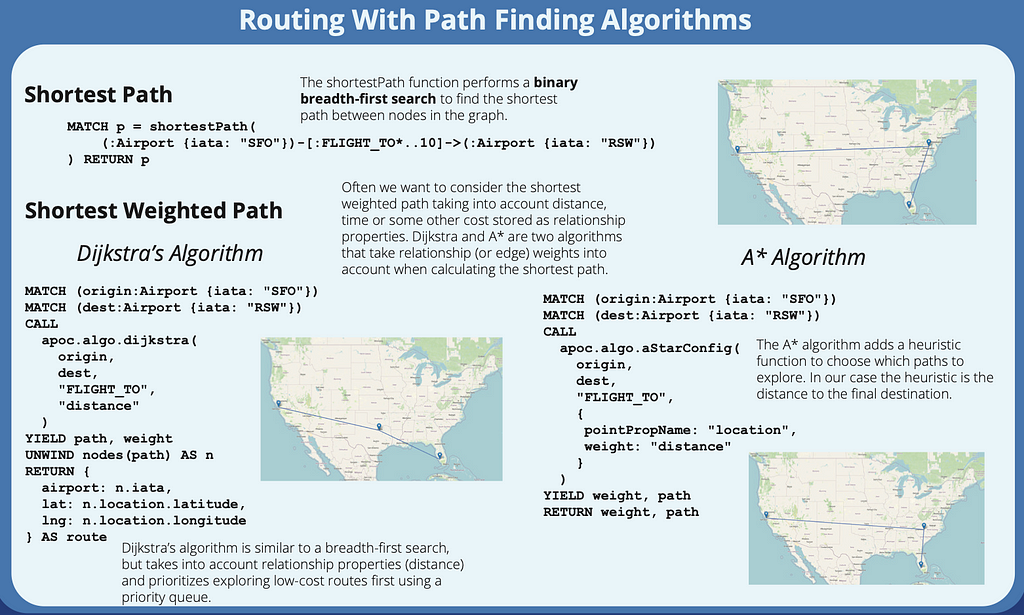
Cypher includes the built-in shortestPath and allShortestPaths function for finding the shortest paths between two nodes. This is good when we want to find the shortest path as measured by the number of relationships to traverse, without considering relationship properties like distance or cost. For our purposes, though we want the shortest weighted path, so we’ll need to use the pathfinding algorithms exposed through the APOC standard library or those available in the Graph Data Science plugin. We’ll use the APOC approach.

Shortest Weighted Path Path Finding Algorithms

Dijkstra’s Algorithm

Dijkstra’s algorithm is typically the one we think of when we think of the “shortest weighted path”. Dijkstra’s algorithm uses a priority queue sorted by cost (or distance in our case) to prioritize exploring the shortest routes.

Here we use Dijkstra’s algorithm to find the shortest route between two address nodes.

MATCH (a:Address)-[:NEAREST_INTERSECTION]->(source:Intersection)
WHERE a.full_address CONTAINS "410 E 5TH AVE SAN MATEO, CA"
MATCH (poi:Address)-[:NEAREST_INTERSECTION]->(dest:Intersection) 
WHERE poi.full_address CONTAINS "39 GRAND BLVD SAN MATEO, CA"
CALL apoc.algo.dijkstra(source, dest, "ROAD_SEGMENT", "length") 
YIELD weight, path
RETURN *

A* Algorithm

A* is an extension of Dijkstra’s algorithm that takes into account a heuristic that measures how close we are getting to the final destination at each step and prioritizes routes that are closer to the destination at each step.

MATCH (a:Address)-[:NEAREST_INTERSECTION]->(source:Intersection)
WHERE a.full_address CONTAINS "410 E 5TH AVE SAN MATEO, CA"
MATCH (poi:Address)-[:NEAREST_INTERSECTION]->(dest:Intersection) 
WHERE poi.full_address CONTAINS "39 GRAND BLVD SAN MATEO, CA"
CALL apoc.algo.aStarConfig(source, dest, "ROAD_SEGMENT", 
  {pointPropName: "location", weight: "length"}) 
YIELD weight, path
RETURN *

Leaflet.js Web Map

Now that we’ve explored options for routing with path-finding graph algorithms let’s see how we can put it all together in a Leaflet.js web map application. We want to allow our users to search for addresses, see them on a map, and view the shortest route from one address to the other.

We’ll use Leaflet to show a map of San Mateo. Above our map we’ll have a text box enabling the user to search for addresses for both the origin and destination of their route.

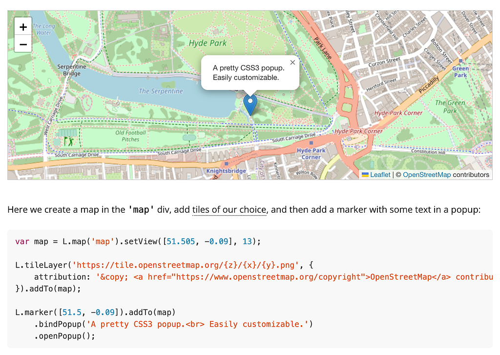
Displaying a Base Map With Leaflet

First we’ll render a base map using Leaflet.js and OpenStreetMap map tiles.

const map = L.map("map", { zoomControl: false }).setView(
 [37.563434, -122.322255],
 13
);

  L.control
    .zoom({
      position: "bottomright",
    })
    .addTo(map);

  const tiles = L.tileLayer(
    "https://tile.openstreetmap.org/{z}/{x}/{y}.png",
    {
      maxZoom: 19,
      attribution:
        '&copy; <a href="https://www.openstreetmap.org/copyright">OpenStreetMap</a>',
    }
  ).addTo(map);

  const popup = L.popup();
  var route = [];

Powering Autocomplete With Full-Text Search

Full-text search indexes in Neo4j allow us to use fuzzy matching across multiple node labels and property values to find matching results. We can use full-text search in Neo4j to power features like autocomplete search results in a web or mobile app.

First, let’s create a full text index combining the Address and PointOfInterest nodes by indexing Address.full_address and PointOfInterest.name This will allow us to search for routing destinations as either addresses or the name of a point of interest.

CREATE FULLTEXT INDEX search_index IF NOT EXISTS 
FOR (p:PointOfInterest|Address) 
ON EACH [p.name, p.full_address]

We search the index by using the db.index.fulltext.queryNodes procedure:

CALL db.index.fulltext.queryNodes("search_index", $searchString) 
YIELD node, score
RETURN coalesce(node.name, node.full_address) AS value, score, labels(node)[0] AS label, node.id AS id
ORDER BY score DESC LIMIT 25

We’ll use this search functionality to enable auto-complete search for each text box.

Drawing A Route on a Leaflet Map

Now we’ll define the Cypher query to use apoc.algo.dijkstra to calculate the route once the user has selected an origin and destination.

const routeQuery = `
  MATCH (to {id: $dest})-[:NEAREST_INTERSECTION]->(source:Intersection) 
  MATCH (from {id: $source})-[:NEAREST_INTERSECTION]->(target:Intersection)
  CALL apoc.algo.dijkstra(source, target, 'ROAD_SEGMENT', 'length')
  YIELD path, weight
  RETURN [n in nodes(path) | [n.location.latitude, n.location.longitude]] AS route
`;

Then when we execute the query we’ll add a marker for the origin and destination and add a polyline to the map to display the route.

var session = driver.session({
          database: "neo4j",
          defaultAccessMode: neo4j.session.READ,
        });

        session
          .run(routeQuery, { source, dest })
          .then((routeResult) => {
            routeResult.records.forEach((routeRecord) => {
              const routeCoords = routeRecord.get("route");
              var polyline = L.polyline(routeCoords)
                .setStyle({ color: "red", weight: 7 })
                .addTo(map);

                console.log(routeCoords[0])
                console.log(routeCoords[routeCoords.length-1])

                var corner1 = L.latLng(routeCoords[0][0], routeCoords[0][1]),
                corner2 = L.latLng(routeCoords[routeCoords.length-1][0], routeCoords[routeCoords.length-1][1])
                
                L.marker(corner1).addTo(map);
                L.marker(corner2).addTo(map);
                
                bounds = L.latLngBounds(corner1, corner2);


              map.panInsideBounds(bounds)
            });
          })
          .catch((error) => {
            console.log(error);
          })
          .then(() => {
            route = [];
            session.close();
          });

Putting it all together we can now search for addresses or points of interest and view the shortest route to them.

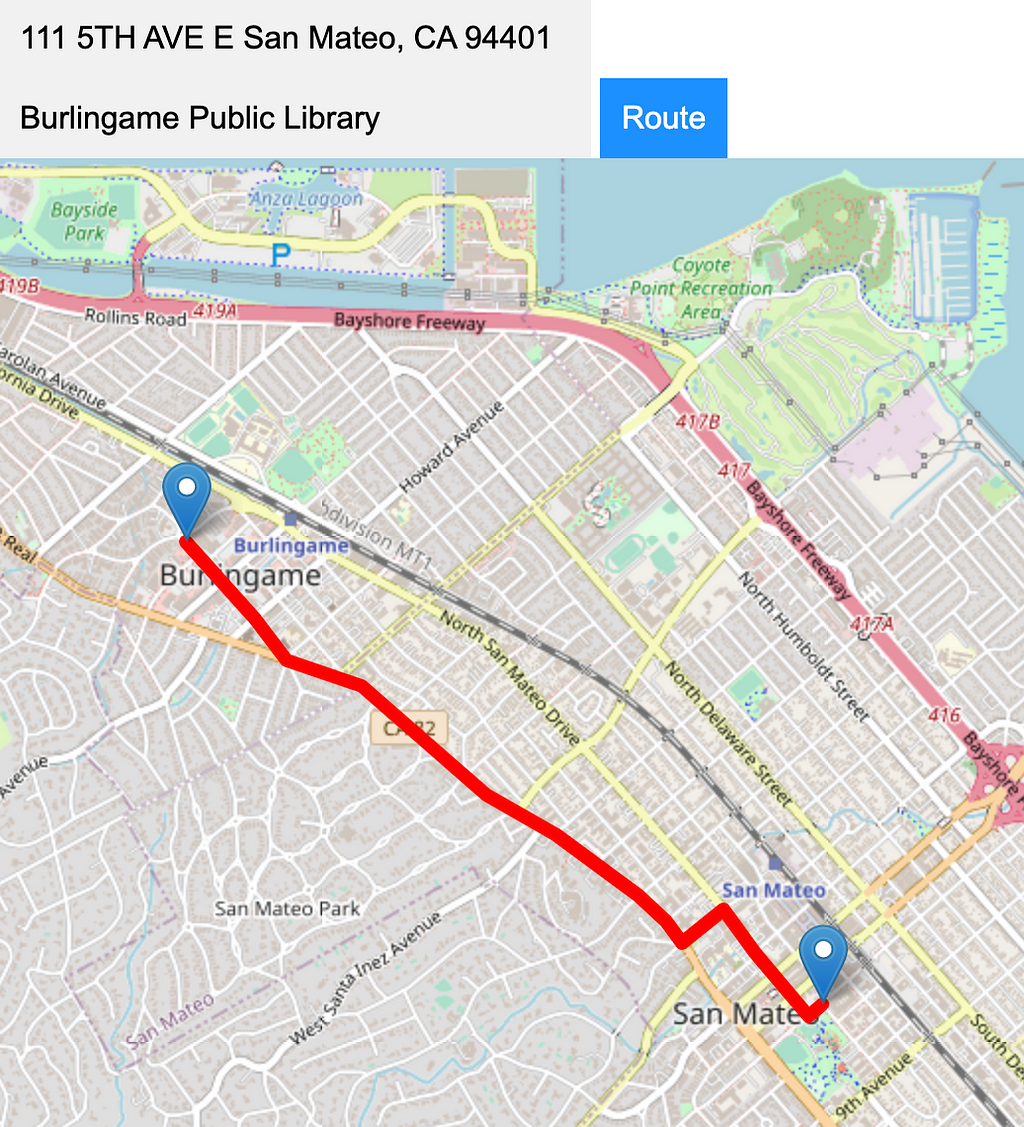
And there we have our basic routing application! Hopefully, this was useful to show how we can use data from OpenStreetMap in Neo4j to build web applications.

If you’re interested in extending this simple application as an exercise, you could add points of interest in addition to addresses or change the Cypher query to use the A* algorithm instead of Dijkstra’s algorithm. Do you get the same results?

Resources

• YouTube recording of the workshop: https://www.youtube.com/watch?v=Z4XZgsbaD9c
• Workshop slides: https://dev.neo4j.com/routing-workshop
• Workshop code on GitHub: https://github.com/johnymontana/openstreetmap-routing-web-app-workshop
• Geospatial graph demos: https://github.com/johnymontana/geospatial-graph-demos
• OSMNx neo4j experiments https://github.com/johnymontana/neo4j-osmnx-experiments

Build a Routing Web App With Neo4j, OpenStreetMap, and Leaflet.js was originally published in Neo4j Developer Blog on Medium, where people are continuing the conversation by highlighting and responding to this story.