


Time Travel with Neo4j Bloom 2.1

Product Manager at Neo4j
8 min read
This week we welcome the release of Neo4j Bloom 2.1, and in this post I’ll showcase a useful new feature – filtering and rule-based styling based on times and dates, which was frequently asked for.

Let’s imagine we wish to analyze some summarized network flow traffic for a global organization with offices in:
- San Francisco (where the timezone offset is GMT-08:00),
- Ottawa (GMT-05:00),
- London (GMT or Z), and
- Malmö (GMT+01:00).
Each office has a network monitoring device, and we’ve loaded data from all of them into our Neo4j database. Our nodes represent internal IP Addresses in the various global offices, and the relationships are traffic flows. The traffic flows have properties indicating the number of packets transferred, to and from ports, the date the sample was collected, and the time the sample was collected – including one of the aforementioned time offsets depending on where the sample was collected.
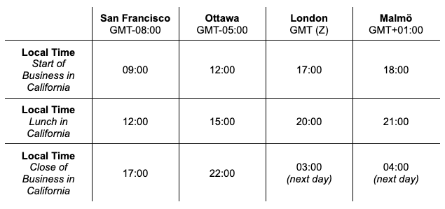
Before we dig any further into our analyses, let’s take a moment to think about the implications of the different time offsets. Consider the table below – we can see what the local time is in each office at certain points in the day – start of business (09:00), lunch (12:00), and close of business (17:00).
While we all understand the concept of time zones, sometimes their impact on visual data analysis is not highly intuitive. An analyst may choose to normalize all times in a dataset to a common time offset like UTC prior to analysis, but this can take extra time and in some cases may not be the ideal solution.
In our case, the time property of a traffic_flow relationship was logged by our network monitoring device and is stored as a time type with the appropriate time offset, depending on the location of the monitoring device.
So, a traffic flow collected at lunchtime in San Francisco (GMT-08:00) would have occurred at 8pm in London (Z). The time property on that relationship would be expressed as 12:00–08:00, to represent that it is 12:00 noon in time zone GMT-08:00 (not 12:00 minus 8 hours).
If data is stored in Neo4j as a temporal value (date, time, localTime, datetime, or localDatetime), Neo4j Bloom now offers the ability to filter and apply rule-based styling to nodes and relationships, including when time zones are present.
There are two ways (default and translated) to apply filters and rule-based styling to properties with time zones (time and datetime values). The features described here also work on temporal values without time zones, albeit without the ability to translate time zones to an offset of choice (more on that later).
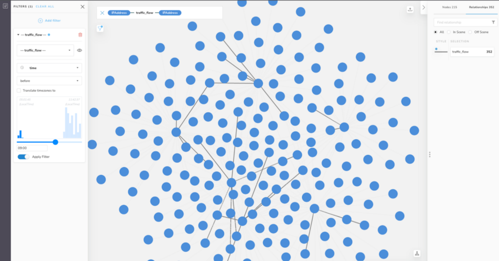
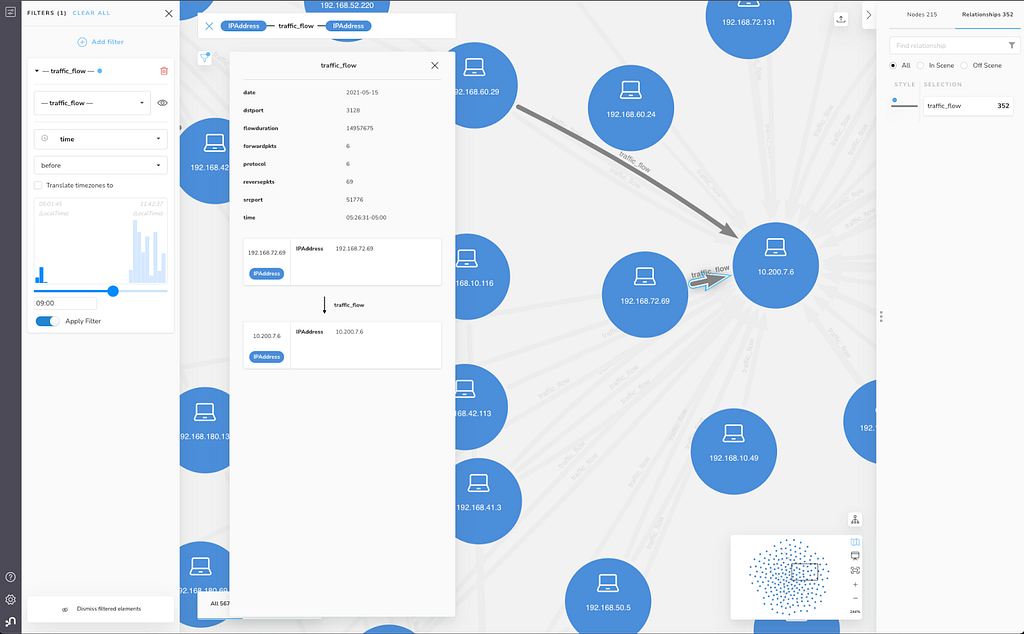
Now, let’s go back to our network data. Here’s a view of IPAddress nodes across our imaginary organization’s four offices, connected by summarized traffic_flow relationships.
A rule-based style has already been applied to the relationships that increases their width according to the number of packets forwarded.
As you can see by the histogram in the Filter pane, the traffic_flow relationships in this scene were all captured between 05:01:45 and 11:42:37. These times do not take the time zones into account – which is to say, they’re local to the office where they were logged by our monitoring devices.
You can see that at the top of the histogram, Bloom shows the earliest time on the left, and the latest time on the right, with LocalTime underneath to show that these are the local times.
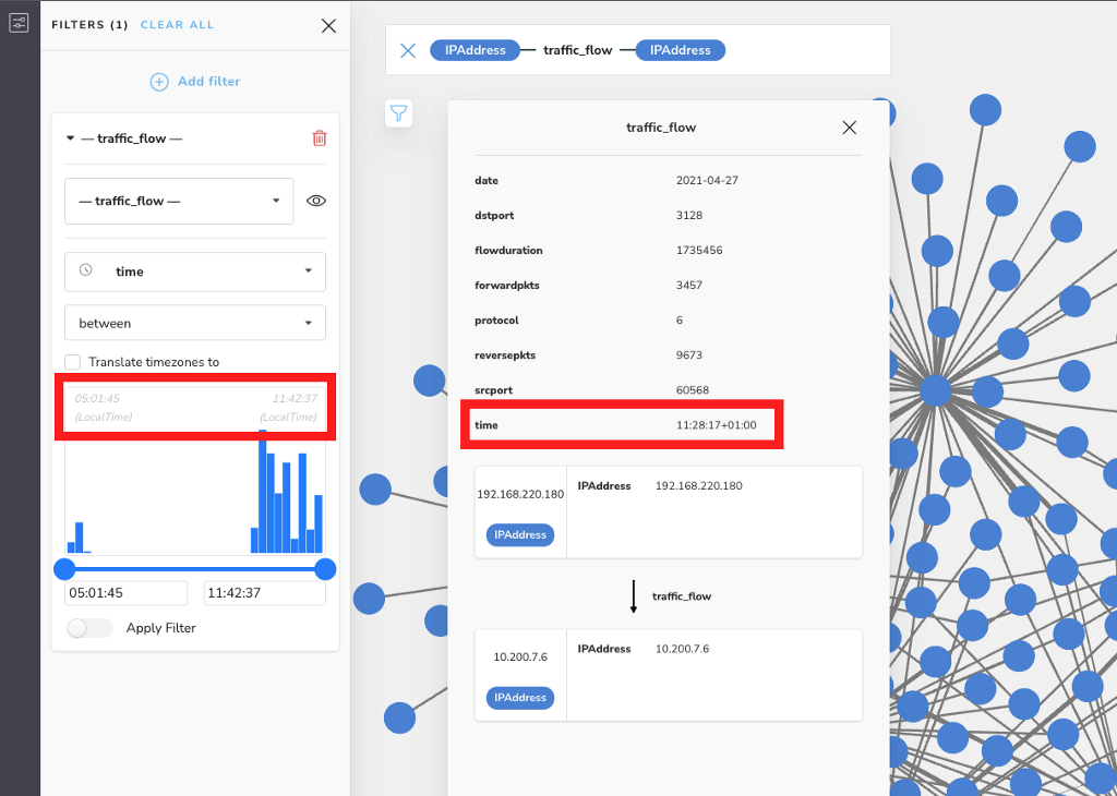
You can also see, in the Inspector, details for one of the traffic_flow relationships, where the time value is 11:28:17+01:00 (indicating this flow was logged by our monitoring device in Malmö, based on the time offset of GMT+01:00). By default, the filter and rule-based style features will ignore the time offset +01:00 for time-zoned data types.
This is useful for certain enquiries. For example, we might want to look at only traffic that occurs before the normal start of business, or 09:00, regardless of where it was collected. Put another way, we want to look at network flows before nine o’clock local time relative to the place where it was logged. Lets simply apply the filter with those criteria:
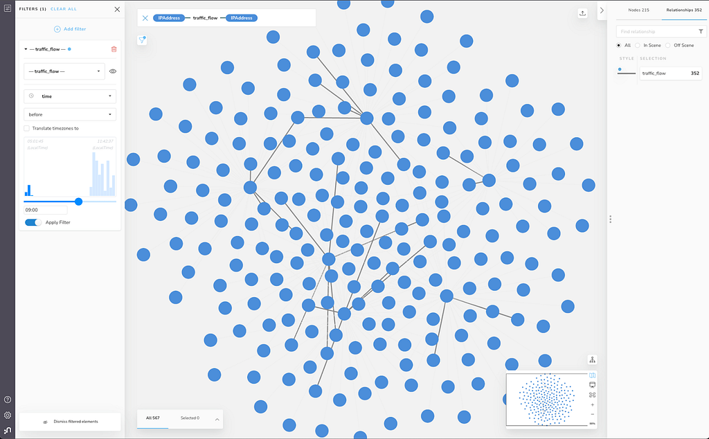
We have significantly reduced the number of traffic_flow relationships visible by applying this filter. We can zoom in and get a closer look at flows of interest.
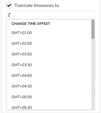
Now, let’s imagine a different type of analytic question. Suppose something anomalous happens with a server in our London office (time offset Z) – maybe it goes offline unexpectedly at around 10:30 local time on a particular day. We can now make use of the Translate timezones to option in Bloom. When selecting this option, a dropdown appears with all possible time offsets.
Neo4j supports only time offsets for
timevalues, but time offsets as well as time zones fordatetimevalues – while the terms are often used interchangeably, including in this post, the difference is simply that time offsets are expressed as GMT + or GMT – some number of hours, whereas time zones are expressed as geographic region names. Bloom will show both in the list fordatetimevalues, but only time offsets fortimevalues.
Since the event we’re concerned with happened around 10:30 in London, we’ll select Z to translate all of the time values in our scene to London time, and look for relationships occurring between 10:25 and 10:35. This will not change the data in the database, nor will it change how that data is displayed in captions or the inspector.
It will only adjust the histogram so that when we select a time, it’s applied to the scene from the perspective of the time offset chosen. You’ll notice that the earliest and latest times are now shown as 10:00:56 and 11:00:56 respectively, because when we translate all of the four different time zones on the scene to London time, everything happened within about the 10:00 to 11:00 window from the perspective of London local time.
What?! Although initially it looked like our data spanned almost seven hours (from about 5 a.m. until almost noon), it really doesn’t – it just appeared that way because, before, we were only looking at the local component of the time values spanning four distant geographic locations (not so intuitive, is it?).
Why don’t the earliest and latest times end with the same minute and second values as before we translated timezones, since we only have four time zones in full-hour increments? That’s because Bloom’s histogram adjusts intelligently to optimize the number of bins and the range for each, based on the data – so changes in the number of bins and their max/min values can be expected when we translate everything to one time zone.
Looking at our table above, we see that there are 12 possible time values if we ignore the time zone (default), with 03:00 being the earliest and 22:00 being the latest. If we normalize all values to, say, GMT-08:00 using ‘Translate timezones to’, then we will only have three values left – 09:00, 12:00, and 17:00. The histogram will adjust accordingly.
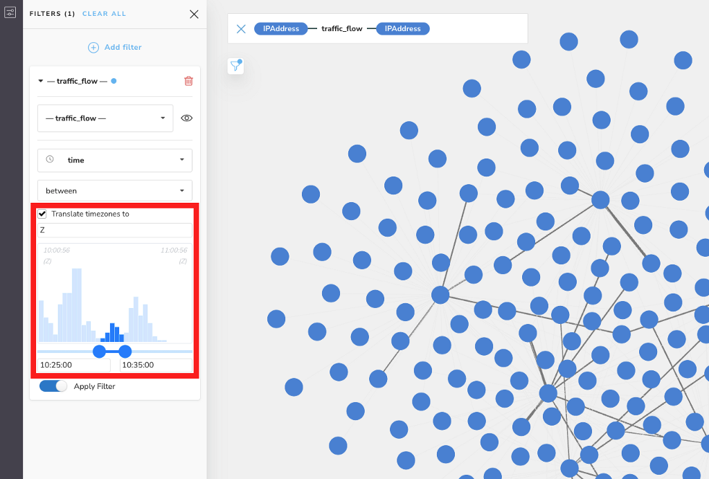
We can now see the flows that happened in this 10-minute interval, regardless of where they were logged. If we zoom in and take a closer look, we see that the time values are still stored and displayed the same way they were before, but we can do the math in our heads to prove that everything is working.
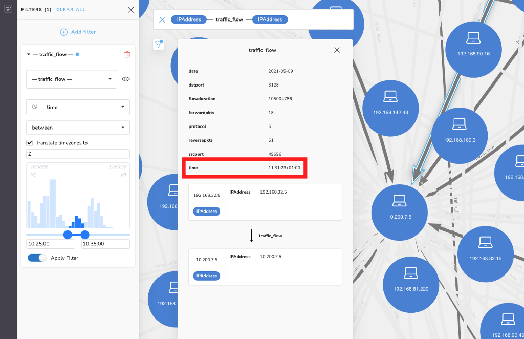
Looking at this particular relationship in the inspector, we see that it was logged at 11:31:23 in GMT+01:00 (based on the time offset, we know it must’ve been logged by the monitoring device in our Malmö office). That means it was 10:31:23 in London at the time (Z) – so it fits within our selected time bounds.
All of these same principles apply in the same way to Bloom’s Rule-based styling, offering a simple way to travel through time in your data analysis. You can even apply some styles and filters with timezone translation, and others without in the same scene, depending on your needs.
If you’re not already a Neo4j Bloom user, feel free to head over to our website and get started by downloading Neo4j Desktop for free, which includes the Basic Access version of Bloom, or set up a free database on AuraDB !
Time Travel with Neo4j Bloom 2.1 was originally published in Neo4j Developer Blog on Medium, where people are continuing the conversation by highlighting and responding to this story.
Share Article


Explore
Related Articles


Architecting Graph-Based Agentic System: When a Regulator Asks “Why Was This Loan Approved?”