Using Neo4j Graph Data Science in Python to improve machine learning models

Graph ML and GenAI Research, Neo4j
18 min read

A wave of graph-based approaches to data science and machine learning is rising. We live in an era where the exponential growth of graph technology is predicted [1]. The ability to analyze data points through the context of their relationships enables more profound and accurate data exploration and predictions. To help you catch the rising wave of graph machine learning, I have prepared a simple demonstration where I show how using graph-based features can increase the accuracy of a machine learning model.
We will be using an anonymized dataset from a P2P payment platform throughout this blog post. The graph schema of the dataset is:
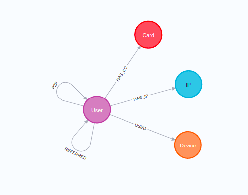
The users are in the center of the graph. Throughout their stay on the P2P platform, they could have used multiple credit cards and various devices from multiple IPs. The main feature of the P2P payment platform is that users can send money to other users. Every transaction between users is represented as the P2P relationship, where the date and amount are described. There could be multiple transactions between a single pair of users going in both directions.
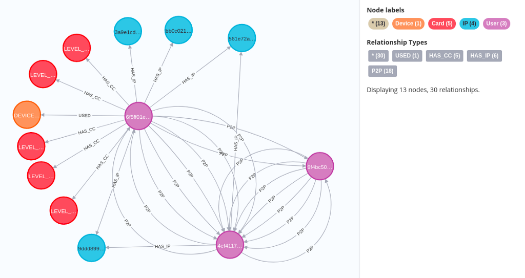
The sample visualization shows users (purple) that can have multiple IPs (blue), Cards (red), and Devices (orange) assigned to them. Users can make transactions with other users, which, as mentioned, is represented as the P2P relationship.
Some of the users are labeled as fraud risks. Therefore, we can use the fraud risk label to train a supervised classification model to perform fraud detection. In this blog post, we will first use non-graphy features to train the classification model, and then in the second part, try to improve the model’s accuracy by including some graph-based features like the PageRank centrality.
All the code is available as a Jupyter Notebook. Let’s dive right into the code!
blogs/p2p-fraud.ipynb at master · tomasonjo/blogs
Prepare the Neo4j environment
We will be using Neo4j as the source of truth to train the ML model. Therefore, I suggest you download and install the Neo4j Desktop application if you want to follow along with the code examples.
The dataset is available as a database dump. It is a variation of the database dump available on Neo4j’s product example GitHub to showcase fraud detection. I have added the fraud risk labels as described in the second part of the Exploring Fraud Detection series, so you don’t have to deal with it. You can download the updated database dump by clicking on this link.
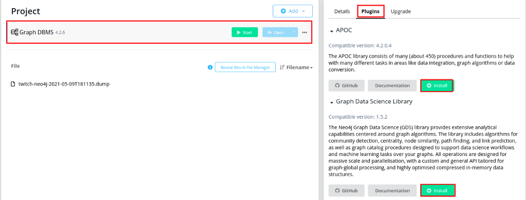
I wrote a post about restoring a database dump in Neo4j Desktop a while ago if you need some help. After you have restored the database dump, you will also need to install the Graph Data Science and APOC libraries. Make sure you are using version 2.0.0 of Graph Data Science or later.
Neo4j Graph Data Science Python client
The Neo4j team released an official Python client for the Graph Data Science library alongside the recent upgrade of the library to version 2.0. Since the Python client is relatively new, I will dedicate a bit more time to it and explain how it works.
First, you need to install the library. You can simply run the following command to install the latest deployed version of the Graph Data Science Python client.
pip install graphdatascience
Once you have installed the library, you need to input credentials to define a connection to the Neo4j database.
In the example I’ve seen, the first thing one usually does is execute the print(gds.version()) line to verify that the connection is valid and the target database has the Graph Data Science library installed.
Exploring the dataset
We will begin with simple data exploration. First, we will count the number of transactions by year from the database using the run_cypher method. The run_cypher method allows you to execute Cypher statements to retrieve data from the database and return a Pandas dataframe.
Results
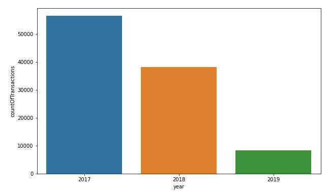
There were more than 50,000 transactions in 2017, with a slight drop to slightly less than 40,000 transactions in 2018. I would venture a guess that we don’t have all the transactions from 2019, as there are only 10,000 transactions available in the dataset.
Our baseline classification model will contain only non-graph-based features. Therefore, we will begin by exploring various features like the number of devices, credit cards, and total and average incoming and outgoing amounts per user. We will stay clear of using the graph algorithm available in the Neo4j Graph Data Science library for now.
We have counted the number of relationships a user has, along with some basic statistics around the incoming and outgoing amounts. First, we will evaluate how many users are labeled as fraud risks. Remember, since the run_cypher method returns a Pandas Dataframe, you can utilize all the typical Pandas Dataframe methods.
Results
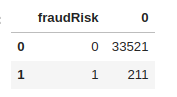
As is typical with the fraud detection scenario, the dataset is heavily imbalanced. One could say that we are searching for a needle in a haystack. Next, we will use the Pandas describemethod to evaluate value distributions.
Results
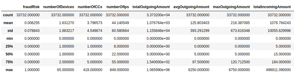
Some of the value distributions are missing from the above results, as they didn’t fit in a single image. You can always look at the full output in the accompanying Jupyter Notebook.
Users have used 1.6 devices on average, with one outlier having used 65 devices. What’s a bit surprising is that the average number of credit cards used is almost four. I think that perhaps the high average of credit cards could be attributed to credit card renewals, and therefore a user needs to add more than one credit card. However, it’s still a higher average than I would expect.
Both the total incoming and outgoing average amounts are around 1,000. Unfortunately, we don’t know the currency or if the transaction values have been normalized, so it is hard to evaluate absolute values. In addition, the median outgoing payment is only five, while the incoming median amount is 15. Of course, there are some outliers as always, as one user has sent over a million through the platform.
Before we move on to training the classification model, we will also evaluate the correlation between features.
Results
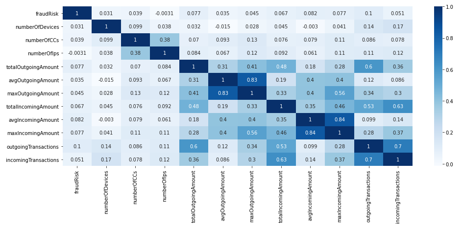
It seems that none of the features correlate with the fraud risk label. As one would imagine, the number of transactions correlates with the total amount sent or received. The only other thing I find interesting is that the number of credit cards correlates with the number of IPs.
Training a baseline classification model
Now it’s time to train a baseline classification model based on the non-graph-based features we pulled from the database. As part of the fraud detection use case, we will try to predict the fraud risk label. Since the dataset is heavily imbalanced, we will use an oversampling technique SMOTE on the training data. We will use Random Forest Classifier to keep things simple, as the scope of this post is not to select the best ML model and/or their hyper-parameters.
I’ve prepared a function that will help us evaluate the model by visualizing the confusion matrix and the ROC curve.
Now that we have the data and the code ready, we can go ahead and train the baseline classification model.
The evaluate function will output confusion matrix, ROC curve, and the feature importance table.
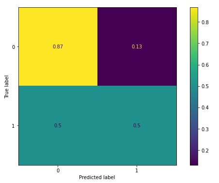
The baseline model features performed reasonably. As a result, it correctly assigned a fraud risk label to 50 percent of the actual fraud risks while misclassifying the other half. Around 13 percent are non-frauds wrongly classified as frauds. Remember, that is quite a considerable number, hence the heavy data imbalance.
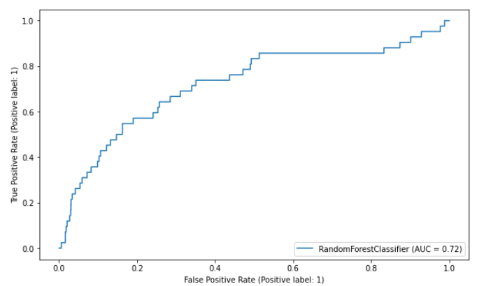
The AUC score of the baseline model is 0.72. The higher the AUC score, the better the model can distinguish between positive and negative labels. Lastly, we will look at the feature importance of the model.
Interestingly, the most important feature is the number of devices — not really what I would expect. I would instead think the that number of credit cards would have a higher impact. The following three important features are all tied to the count and the amount of the incoming transactions.
Using graph-based features to increase the accuracy of the model
In the second part of the post, we will use graph-based features to increase the performance of the classification model. Lately, graph neural networks and various node embedding models are gaining popularity. However, we will keep it simple in this post and not use any of the more complex graph algorithms. Instead, we will use more classical centrality and community detection algorithms to produce features that will increase the accuracy of the classification model.
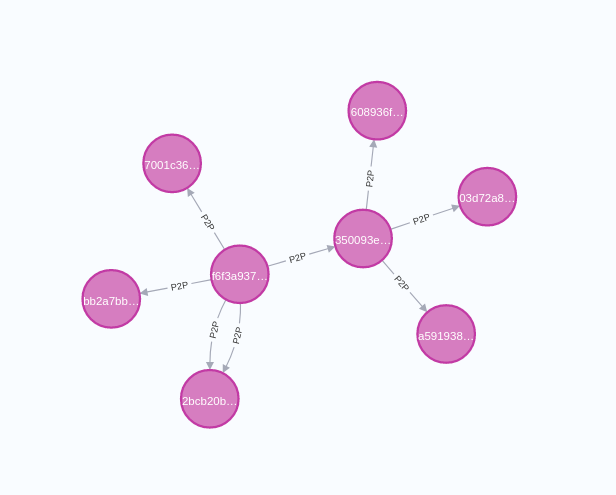
We have a couple of networks in our dataset. First, there is a direct P2P transaction network between users that we can employ to extract features that describe users.
On the other hand, there are also indirect connections between users, where some users use the same device, IP, or credit card.
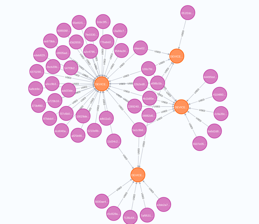
The above image visualizes a network of users (purple) and devices (orange) they have used. For example, it might be that the left device used by a high number of users could be a public computer in a library or a coffee shop. It is also not unusual for family members to use the same device.
In our example, we will use the P2P transaction network between users and indirect connections between users who share credit cards as the input to graph algorithms to extract predictive features.
Before executing any graph algorithms, we have to project the Graph Data Science in-memory graph. We will be using the newly released Graph Data Science Python client to project an in-memory graph. The Python client mimics the Graph Data Science Cypher procedure and follows an almost identical syntax. It seems to me that the only difference is we don’t prefix the Cypher procedures with the CALLoperator as we would when, for example, executing graph algorithms in Neo4j Browser.
We can use the following command to project User and Card nodes along with the HAS_CC and P2P relationships.
For those of you who have experience with Graph Data Science, or read my previous blog post, the projection definition is, for the most part, straightforward. The only thing I haven’t used in a while is merging parallel P2P relationships into a single relationship during projection and summing their total amount. We merge parallel relationships and sum a specific property of the relationships using the following syntax:
'P2P':{
    'type':'P2P',
    'properties':{
        'totalAmount':{
             'aggregation':'SUM'
         }
     }
}
You can observe the following visualization to understand better what the above syntax does.
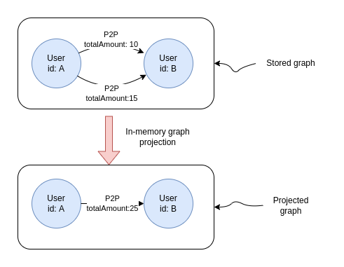
With the projected in-memory graph ready, we can go ahead and execute intended graph algorithms.
Weakly connected components
We will begin by using the Weakly Connected components (WCC) algorithm. The WCC algorithm is used to find disconnected components or islands within the network.
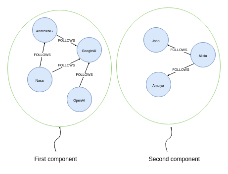
All nodes in a single weakly connected component can reach other nodes in the component when we disregard the direction of the relationship. The above example visualizes a network where two components are present. There are no connections between the two components, so members of one component cannot reach the members of the other component.
In our example, we will use the WCC algorithm to find components or islands of users who used the same credit card.
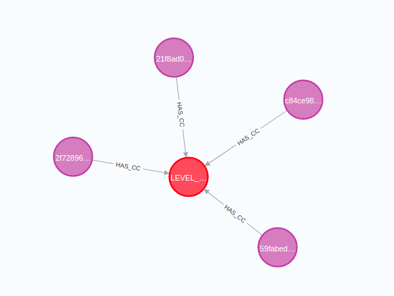
In this example, we have four users who used the same credit card. Therefore, the Weakly Connected component algorithm that considers both users and their credit cards will identify that this component contains four users.
We will use the stream mode of the WCC algorithm using the GDS Python client, which will return a Pandas Dataframe. Any additional configuration parameters can be added as keyword arguments.
We have used the nodeLabels parameter to specify which nodes the algorithm should consider, as well as the relationshipTypes parameter to define relationship types. Using the relationshipTypes parameter, we have defined the algorithm to consider the HAS_CC relationships and ignore the P2P relationships.
As mentioned, the above statement returns a Pandas Dataframe that contains the internal node ids and the component ids.
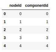
The output of the WCC algorithm will contain both the User and the Card nodes. Since we are only interested in User nodes, we must first retrieve the node labels using the gds.util.asNodes method and then filter on the node label.
Lastly, we will define two features based on the WCC algorithm results. The componentSize feature will contain a value of the users in the component, while the part_of_community feature will indicate if the component has more than one member.
PageRank centrality
Next, we will use the PageRank centrality of the P2P transaction network as one of our features. PageRank algorithm is commonly used to find the most important or influential nodes in the network. The algorithm considers every relationship to be a vote of confidence or importance, and then the nodes deemed the most important by other important nodes rank the highest.
Unlike the degree centrality, which only considers the number of incoming relationships, the PageRank algorithm also considers the importance of nodes pointing to it. A simple example is that being friends with the president of the country or a company gives you more influence than being friends with an intern. Unless that intern happens to be a family relative to the CEO.
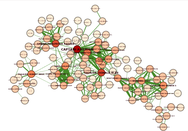
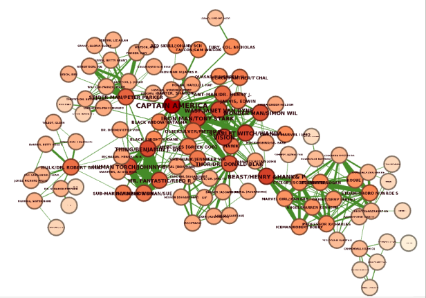
In this visualization, nodes are colored based on their PageRank score, with the red color indicating the highest rank and the white color indicating the lowest score. For example, Captain America has the highest PageRank score. Not only does he have a lot of incoming relationships, but he also has connections with other important characters like Spider Man and Thor.
You can execute the stream mode of the weighted variant of the PageRank algorithm using the following Python code.
This code first executes the stream mode of the PageRank algorithm, which returns the results in the form of the Pandas Dataframe. Using the nodeLabels parameter, we specify that the algorithm should only consider User nodes. Additionally, we use the relationshipTypes parameter to use only the P2P relationships as input. Lastly, we merge the new PageRank score column to the graph_features dataframe.
Closeness centrality
The last feature we will use is the Closeness centrality. The Closeness centrality algorithm evaluates how close a node is to all the other nodes in the network. Essentially, the algorithm results inform us which nodes can reach all the other nodes in the network the fastest.
This visualization contains the same network I used for the PageRank centrality score. The only difference is that the node’s color depends on their Closeness centrality score. We can observe that the nodes in the center of the network have the highest Closeness centrality score, as they can reach all the other nodes the fastest.
The syntax to execute the Closeness centrality and merge the results to the graph_features data frame is almost identical to the PageRank example.
Combine baseline and graph features
Before we can train the new classification model, we have to combine the original dataframe that contains the baseline features with the graph_feature dataframe that includes the graph-based features.
The original dataframe does not contain the internal node ids, so we must first extract the user ids from the node object column. Next, we can use the user id column to merge the baseline and the graph-based feature dataframes.
Include the graph-based features in the classification model
Now we can go ahead and include both the baseline as well as the graph-based features to train the fraud detection classification model.
First, we can take a look at the confusion matrix.
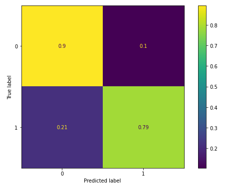
We can observe that the model correctly classified 79 percent of fraudsters, rather than the 50 percent with the baseline model. However, it also misclassifies fewer non-frauds as frauds. We can observe that the graph-based features helped improve the classification model accuracy.
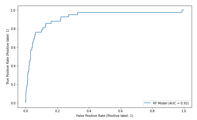
We can also observe that the AUC score has risen from 0.72 to 0.92, which is a considerable increase.
Finally, let’s evaluate the importance of the graph-based features.
While the number of credit cards used by a user might be significant to classify the fraudsters accurately, a far more predictive feature in this dataset is looking at multiple users and how many used those credit cards. The PageRank and Closeness centrality also added a slight increase in the accuracy, although they are less predictive in this example than the Weakly Connected component size.
Conclusion
Sometimes a more extensive dataset or more annotated labels can help you improve the machine learning model accuracy. Other times, you need to dig deeper into the dataset and extract more predictive features.
If your datasets contain any relationships between data points, it is worth exploring if they can be used to extract predictive features to be used in a downstream machine learning task. We’ve used simple graph algorithms like centrality and community detection in this example, but you can also dabble with more complex ones like graph neural networks or node embedding models. I hope to find more scenarios where more complex algorithms come into play and then write about them.
In the meantime, you can start exploring your datasets with the Neo4j Graph Data Science library and try to produce predictive graph-based features. As always, all the code is available on GitHub.
References
Using Neo4j Graph Data Science in Python to Improve Machine Learning Models was originally published in Neo4j Developer Blog on Medium, where people are continuing the conversation by highlighting and responding to this story.
Share Article


Explore
Related Articles
Hybrid Search in Neo4j: Full-Text, Vectors, and Graph Topology with Cypher