Discover AuraDB Free: Week 17 – Analyzing NFT Trades

This week we used a subset of a published NFT Trades dataset to model, import, and analyze in Neo4j AuraDB Free.

If you missed our recording here it is (sorry for the audio issues):

It all started with a Tweet that I came across one late night about a research paper on NFT trades.

NFT oligarchy? A study of 6.1M NFT trades finds a few folks at the center of the market
? The top 10% of traders account for 85% of transactions & trade at least once 97% of all assets
?10% of buyer–seller pairs have the same volume as the remaining 90% https://t.co/V3vytqZZB5 pic.twitter.com/IDr67zl7TI
— Ethan Mollick (@emollick) November 30, 2021

Fortunately the authors also published the accompanying data, a whopping 6.1M trades in a CSV format.

I spent a bit of time running full data import with the data importer tool and looking at the data.

Thanks for sharing the thread, and to the authors for making the data available. Saw the tweet and did a quick import into #Neo4j, if anyone wants to play with the data. https://t.co/qyk9IYaw5G pic.twitter.com/QYSaVT0Xfe
— Michael Hunger (@mesirii) December 1, 2021

After sharing the dataset with @Tomaz.Bratanic, he took it even further, cleaning it up and doing a proper analysis that he published on TowardsDataScience. It’s a really insightful article, but even that still just scratches the surface of the data.

Exploring the NFT transaction with Neo4j

Dataset

The full CSV data set is too large for the limits of AuraDB Free — 3.8GB uncompressed CSV with 6M rows (it has 7.9M lines due to many descriptions with newlines).

That’s why we look at a single day of trades, Jan 1, 2021, which has 5119 rows and is 3.6MB large.

If you want to analyze a larger portion of the data, feel free to use an AuraDB Pro instance (paid) or Download Neo4j Desktop.

We used xsv to filter the data down, and published the small CSV file to GitHub for you to download.

xsv search -s 'Datetime_updated' '2021-01-01'  Data_API.csv | xsv count
    5119
xsv search -s 'Datetime_updated' '2021-01-01'  Data_API.csv  > nft_2021-01-01.csv

xsv frequency -s Market nft_2021-01-01.csv

field,value,count
Market,Atomic,3214
Market,OpenSea,1857
Market,Cryptokitties,25
Market,Godsunchained,19
Market,Decentraland,4

Model

The model is pretty straightforward, with a few small tweaks.

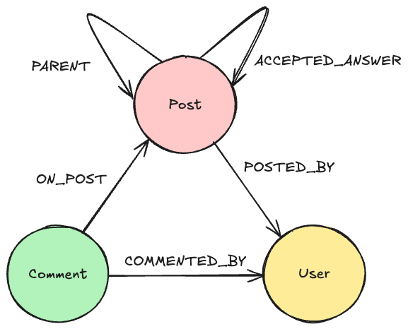
We have an NFT which is in a Category and Collection. It is traded in a Transaction for this NFT, sold by a Seller, and bought by a Buyer, both of which are also Trader.

The unique id’s for NFT are ID_token, for Traders their equivalent addresses and for the Transaction it’s the transaction_hash. (Actually during the livestream we learned that Unique_id_collection is a better fit as ID_token has duplicates across markets.)

Data Import

We use the data importer tool for a quick and easy modeling and data import run.

TLDR; If you don’t want to draw the model yourself we also have prepared a model + CSV archive that you can load directly with this link to the data importer.

Load the CSV
Create the graph model
Map the same file time and again to the different nodes and relationships

I labeled the Buyer and Seller both Trader and removed the prefix from buyer_address and buyer_username field-names, so that they are uniquely created once, no matter the role they have in a transaction.

We mostly mapped the other properties directly to the different nodes (don’t forget to select the id-fields!) and for the relationships select the appropriate id-field for each node.

We need to convert the currency fields Price_USD and Price_Crypto to floating point numbers.

After all elements have gotten their blue checkmarks and all the columns in the CSV file are green, you can proceed to the import.

Neo4j AuraDB Free

Create a new Neo4j AuraDB Free instance, e.g. called NFT, make sure to save the password.

The database takes 2–3 minutes to be provisioned, and after it is running you also need the connection URL.

Run Import

With the connection information, go back to the data importer and click “Run Import.”

Put in the details and click run.

Afterwards you’ll see the the result overview with the runtime and can look at each import statement.

Neo4j Browser and Bloom

In the AuraDB UI you can “Open” your database with Neo4j Browser a Graph Query UI that allows you to run statements, visualize the results as graphs and tables. This is where we will do our post-processing.

With Neo4j Bloom, you can explore and visualize the data without needing to know Cypher.

For both, you will need your saved password to log in.

Post Processing

And we need to post convert the Datetime_updated and Datetime_updated_seconds to datetime format, which the data importer doesn’t yet support.

MATCH (t:Transaction)
SET t.Datetime_updated =
    datetime(replace(t.Datetime_updated,' ','T'))
SET t.Datetime_updated_seconds =
    datetime(replace(t.Datetime_updated_seconds,' ','T'));

For Trader nodes that have a SOLD relationship, we set the Seller label, similar for Buyer. Some Traders will have both.

MATCH (t:Trader)
WHERE exists { (t)-[:SOLD]->() }
SET t:Seller;

MATCH (t:Trader)
WHERE exists { (t)-[:BOUGHT]->() }
SET t:Buyer;

Data Exploration

Let’s look at the data at a high level. Remember we only imported one day of trades, so the whole dataset is much more insightful.

Number and volume of trades:

MATCH (t:Transaction)
RETURN count(*) as count, round(sum(t.Price_USD)) as volumeUSD;

Which gives us an impressive half-a-million dollars in trades on New Year’s day of 2021 in only 1871 trades.

╒═══════╤═══════════╕
│"count"│"volumeUSD"│
╞═══════╪═══════════╡
│1871   │521768.0   │
└───────┴───────────┘

We will follow Tomaz’ blog post and only share a few of the queries here, so you can also copy the queries from there and read his analysis.

Exploring the NFT transaction with Neo4j

NFTs sold at the highest price:

MATCH (n:NFT)<-[:FOR_NFT]-(t:Transaction)
WHERE exists(t.Price_USD)
WITH n, t.Price_USD as price
ORDER BY price DESC LIMIT 5
RETURN price, n.ID_token as token_id, n.Image_url_1 as image_url

Pretty impressive prices – 65k, 33k, and around 15k for pretty ugly images (if you follow the links).

Traders with the highest transaction count and volume:

MATCH (t:Trader)
OPTIONAL MATCH (t)-[:BOUGHT]->(bt)
WITH t, round(sum(bt.Price_USD)) AS boughtVolume, count(*) as buys
OPTIONAL MATCH (t)-[:SOLD]->(st)
WITH t, boughtVolume, buys,
     round(sum(st.Price_USD)) AS soldVolume, count(*) as sales
RETURN
       t.address AS address,
       boughtVolume, buys,
       soldVolume, sales
ORDER BY buys + sales
DESC LIMIT 6;

Here we see clearly pure sellers (artists?), buyers, and some traders that buy and sell. Remember that this is only a single day.

╒════════════~════════╤════════╤══════╤═══════╤═══════╕
│"address"            │"bought"│"buys"│"sold" │"sales"│
╞════════════~════════╪════════╪══════╪═══════╪═══════╡
│"0x327305a79~2b1a8fa"│0.0     │1     │25314.0│253    │
├────────────~────────┼────────┼──────┼───────┼───────┤
│"0xab5853ddb~703f5be"│18443.0 │52    │0.0    │1      │
├────────────~────────┼────────┼──────┼───────┼───────┤
│"0x95a437e4c~5e25d81"│110.0   │1     │1436.0 │33     │
├────────────~────────┼────────┼──────┼───────┼───────┤
│"0x709a911d6~f24aef9"│0.0     │1     │210.0  │25     │
├────────────~────────┼────────┼──────┼───────┼───────┤
│"0x75dffacbc~5322c4e"│481.0   │17    │265.0  │5      │
├────────────~────────┼────────┼──────┼───────┼───────┤
│"0x68aef8296~e111d0b"│0.0     │1     │264.0  │18     │
└────────────~────────┴────────┴──────┴───────┴───────┘

We can also compute the highest profit someone made on this day:

MATCH (t:Trader)-[:SOLD]->(st:Transaction)-[:FOR_NFT]->(nft)
WHERE st.Price_USD > 1000
MATCH (t)-[:BOUGHT]->(bt:Transaction)-[:FOR_NFT]->(nft)
WHERE st.Datetime_updated_seconds > bt.Datetime_updated_seconds
RETURN coalesce(t.username, t.address) as trader,
       nft.Image_url_1 as nft,
       nft.ID_token AS tokenID,
       st.Datetime_updated_seconds AS soldTime,
       round(st.Price_USD) AS soldAmount,
       bt.Datetime_updated_seconds as boughtTime,
       round(bt.Price_USD) AS boughtAmount,
       round(st.Price_USD - bt.Price_USD) AS difference
ORDER BY difference DESC LIMIT 5

We find only one trader who sold something for more than 1000 USD and they made a nice 4867 USD profit.

trader: Korniej
tokenID: 8000067
boughtAmount: 367.0
soldAmount: 5134.0
difference: 4767.0
boughtTime: 2021–01–01T18:58:35Z
soldTime: 2021–01–01T19:47:48Z

For this NFT, not bad heh 🙂

Example Picture of NFT sold for 5134.0 Jan 01 2021

Another interesting aspect are traders with self loops, as exemplified by this statement:

MATCH p=(t:Trader)-[:BOUGHT]->()<-[:SOLD]-(t)
RETURN p LIMIT 10

Or traders that repeatedly occurred in the same transaction:

MATCH p=(t1:Trader)-[:BOUGHT]->()<-[:SOLD]-(t2)
WITH t1, t2, count(*) as c
ORDER BY c DESC
LIMIT 5
RETURN substring(t1.address,0,10) as t1, 
       substring(t2.address,0,10) as t2, c

So on the same day some folks traded several times with each other:

╒════════════╤════════════╤═══╕
│"t1"        │"t2"        │"c"│
╞════════════╪════════════╪═══╡
│"0x7e9e93d7"│"0x68aef829"│16 │
├────────────┼────────────┼───┤
│"0xa0f80f5c"│"0x327305a7"│9  │
├────────────┼────────────┼───┤
│"0x75dffacb"│"0x327305a7"│8  │
├────────────┼────────────┼───┤
│"0x8d09aeac"│"0xfd62e6db"│6  │
├────────────┼────────────┼───┤
│"0x010bc884"│"0x6958f5e9"│6  │
└────────────┴────────────┴───┘

Data Visualization

With Neo4j Bloom we can look at the data visually, even the whole dataset of 9886 nodes and 19944 relationships.

You can just open Neo4j Bloom from the AuraDB’s “Open” button drop-down.

You can look at co-buying behavior by entering the phrase.

“Seller Transaction NFT”

Right click and choose “Clear Scene” to remove the current visualization – otherwise it’s additive.

You can also look at collections of NFTs with the search phrase “Collection NFT.”

We can also style the transactions based on volume and cryptocurrency.

Pick the “Transaction” entry in the right side legend and choose “Rule-Based-Styling”:

Price_USD
Size
Range
Refresh Range
0.25x to 4x
Apply

Then you can do the same for the color by adding another rule, going for:

Market
Color
Unique Values
Apply

So you can see the transactions stand out by volume and immediately spot the market they were on.

Conclusion

This only scratches the surface of what you can do with the data.

You can query and analyze more
Visualize more intricate relationships
Add new data and computed relationships
Run graph algorithms
Write apps that allow people to search for and visualize NFT trades

Let us know what you come up with.

Happy graphing!

Get started with Neo4j AuraDB Free now. No download required.

Try Neo4j AuraDB Free Now

Resources

Discover AuraDB Free: Week 17 – Analyzing NFT Trades was originally published in Neo4j Developer Blog on Medium, where people are continuing the conversation by highlighting and responding to this story.

AuraDB freeCloudcryptocryptocurrencydata vizdata-analysisethereumgraph-databasehow-toNeo4jnfttransactionsvisualization

GRAPH TOOLS

DEVELOPERS

DATA SCIENTISTS

LEARN

CONNECT

FEATURED EVENTS

QUICK LINKS

Hear directly from data and business trailblazers

Join our online conference. New themes every time.

Discover AuraDB Free: Week 17 – Analyzing NFT Trades

Michael Hunger, Developer Relations Jan 31, 2022 7 mins read