Use Neo4j Parallel Spark Loader to Improve Large-Scale Ingestion Jobs

Consulting Engineer, Neo4j
14 min read

Create relationships in parallel
In this blog, we’ll detail some common issues that occur during parallel ingestion into a graph. We’ll cover how the Neo4j Parallel Spark Loader Python package eliminates these issues and provides enhanced performance at high data volumes. This package and article were written by Nathan Smith and myself.
This article was written for v0.4.0 of the Neo4j Parallel Spark Loader. All benchmarking results are gathered using this version of the library.
Neo4j
Neo4j is a transactional graph database that uses nodes, relationships, and properties to represent data. It offers high scalability and ACID compliance, and uses the Cypher query language to interact with data within the graph. Learn about the Neo4j cloud-based solution, AuraDB.
Apache Spark
Apache Spark is a tool often used to work with big data on clusters. Spark is a key piece of many cloud data services, including Databricks, Azure Synapse Analytics, Amazon Elastic MapReduce (EMR), AWS Glue, and Google Cloud Dataproc. Neo4j Connector for Apache Spark allows users load data from Spark DataFrames to Neo4j. Spark can easily distribute data across multiple servers in a cluster, and with the Neo4j Connector for Apache Spark, the distributed data can be sent to Neo4j in parallel transactions. This makes Spark a great choice for efficiently loading data to Neo4j.
Background
A common issue that developers run into when ingesting their data into a graph database is handling deadlocks. Deadlocks occur when multiple transactions attempt to modify the same data at the same time. This commonly occurs during ingestion when two different relationships have a shared node as the source or target. If these two relationships are loaded in parallel, a deadlock error will occur and the ingestion will fail.
There are simple ways to combat this issue. You may implement a retry loop that waits a certain amount of time for each failed write before retrying the transaction. They may also write all relationships serially at the cost of additional ingestion time. While these approaches may be successful, they are still prone to failure or incur additional time spent ingesting data.
Solution
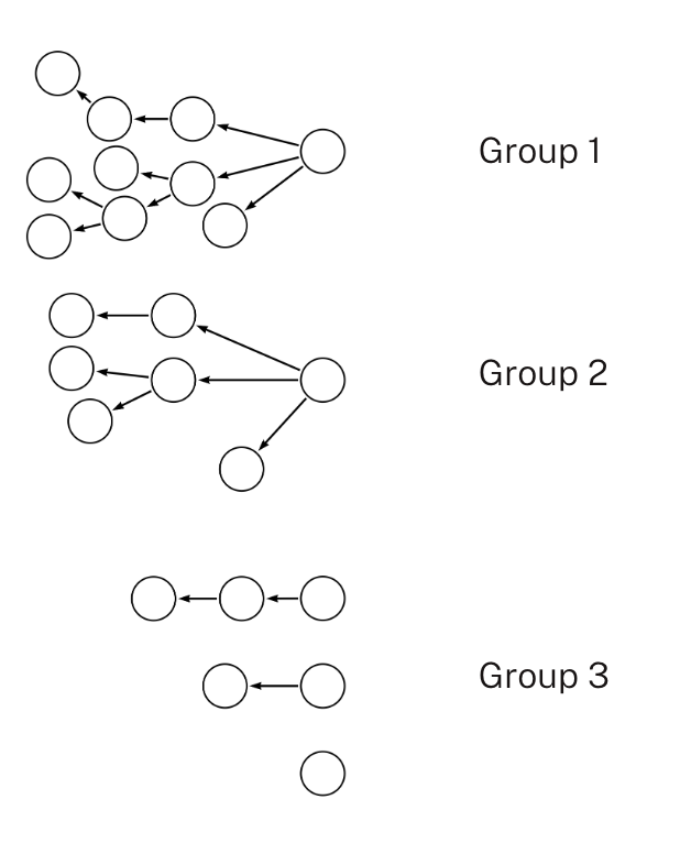
The Neo4j Parallel Spark Loader Python package implements a solution to this problem that was described in Mix and Batch: A Technique for Fast, Parallel Relationship Loading in Neo4j by Eric Monk. This solution identifies groups of relationships where no nodes are endpoints of relationships in more than one group. These relationship groups can then be loaded in parallel without the risk of deadlocking. In some graph topologies, it’s not possible to partition all relationships into a desired number of groups with no shared endpoints. In these cases, multiple batches may be created, with each batch containing non-overlapping groups. All the groups in the first batch can then be loaded in parallel, then groups in the second batch may be loaded, etc. This allows relationships to be loaded in parallel and improve ingestion time at the cost of some additional preprocessing in the beginning.
It is most efficient if the groups within each batch are roughly equal in size. That way, a small group in a batch doesn’t finish quickly, leaving Spark resources idle while a larger group in the same batch completes. The Neo4j Parallel Spark Loader can assign relationships to balanced groupings, or you can provide your own relationship groupings if they can be easily derived from your source data.
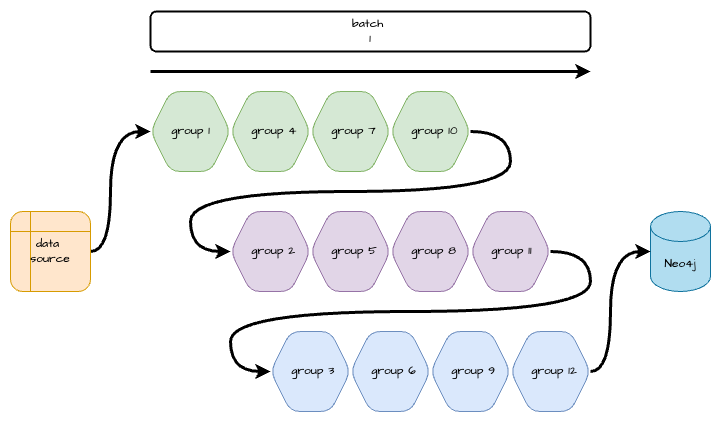
The diagram below details a serial workflow where each group of relationships must be ingested one after the other to avoid deadlocking.
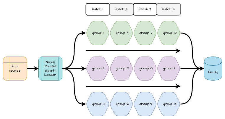
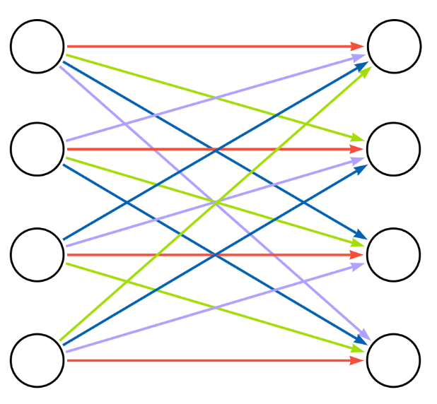
The next diagram details a parallel workflow that batches the groups appropriately so they may be ingested simultaneously without causing deadlocks.
Python Package
The Neo4j Parallel Spark Loader Python package addresses the issue of loading relationships in parallel with the solution above. This is done by using Spark’s Python wrapper library, PySpark, to determine appropriate groups and batches and ingest the data in parallel. It requires some basic knowledge of how Spark works as well as an understanding of the underlying graph structure contained in the relationships of interest. We’ll walk through some examples and explain the possible graph structures.
The package may be installed with pip install neo4j-parallel-spark-loader
Graph Structures
Depending on the structure of the relationship data being loaded to Neo4j, grouping and batching scenarios of various levels of complexity can be appropriate. The Neo4j Parallel Spark Loader library supports three scenarios: predefined components, bipartite data, and monopartite data.
Each grouping and batching scenario has its own module. The group_and_batch_spark_dataframe() function in each module accepts a Spark DataFrame with parameters specific to the scenario. It appends batch and group columns to the DataFrame. The ingest_spark_dataframe() function splits the original DataFrame into separate DataFrames based on the value of the batch column. Each batch’s DataFrame is repartitioned on the group column and written to Neo4j with Spark workers processing groups in parallel.
Predefined Components
In some relationship data, relationships can be broken into distinct components based on a field in the relationship data. For example, a DataFrame of HR data has columns for employeeId, managerId, and department. If a MANAGES relationship between employees and managers is needed, and it is known in advance that all managers are in the same department as the employees they manage, the rows of the DataFrame may be separated into components based on the department key.
The number of predefined components is often greater than the number of workers in the Spark cluster, and the number of rows within each component is unequal. When running parallel_spark_loader.predefined_components.group_and_batch_spark_dataframe(), the number of groups you want to collect the partitioned data into is specified as an argument. This value should be less than or equal to the number of executors in your Spark cluster. Neo4j Parallel Spark Loader uses a greedy algorithm to assign partitions into groups in a way that attempts to balance the number of relationships within each group. When loading, this ensures that each Spark worker stays equally, instead of some workers waiting while other workers finish loading larger groups.
The following diagram shows how each group contains no overlapping nodes with another group. This allows the three groups to be loaded in parallel.
Bipartite
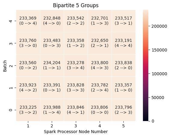
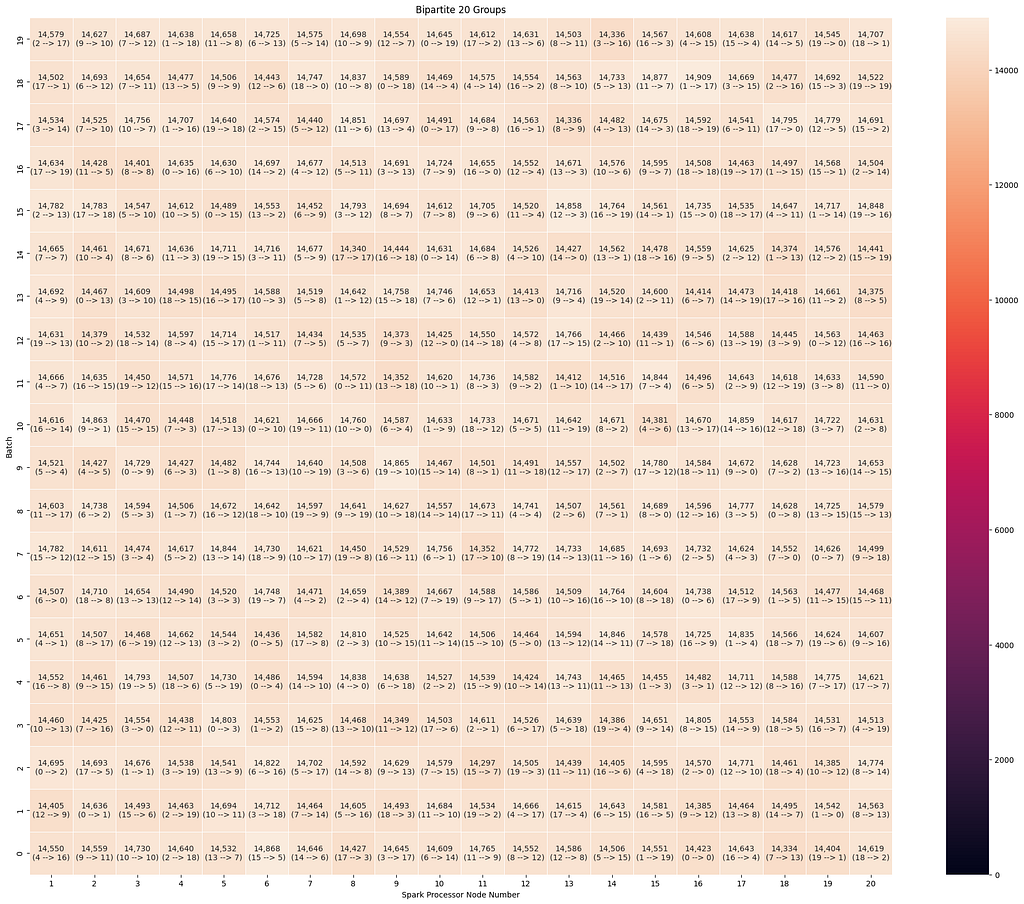
In many relationship datasets, there isn’t a partitioning key in the Spark DataFrame that can divide the relationships into predefined components. However, it is known that no nodes in the dataset will be both a source and a target for this relationship type. This is usually because the source nodes and the target nodes have different node labels, and they represent different classes of things in the real world. For example, a DataFrame of order data might have columns for orderId, productId, and quantity, and need INCLUDES_PRODUCT relationships between Order and Product nodes. Here, all source nodes of INCLUDES_PRODUCT relationships will be Order nodes, and all target nodes will be Product nodes. No nodes will be both source and target of that relationship.
When running parallel_spark_loader.bipartite.group_and_batch_spark_dataframe(), the number of groups the source and target nodes should be collected into isan argument. This value should be less than or equal to the number of executors in your Spark cluster. Neo4j Parallel Spark Loader uses a greedy algorithm to assign source node values to source-node groups so that each group represents roughly the same number of rows in the relationship DataFrame. Similarly, the library groups the target node values into target-node groups with roughly balanced sizes.
We can visualize the nodes within the same group as a single aggregated node and the relationships that connect nodes within the same group as a single aggregated relationship.
In the aggregated bipartite diagram, multiple relationships (each representing a group of individual relationships) connect to each node (representing a group of nodes). Using a straightforward alternating algorithm, the relationships are colored so that no relationships of the same color point to the same node. The relationship colors represent the batches applied to the data. In the diagram above, the relationship groups represented by red arrows can be processed in parallel because no node groups are connected to more than one red relationship group. After the red batch completes, each additional color batch can be processed in turn until all relationships have been loaded.
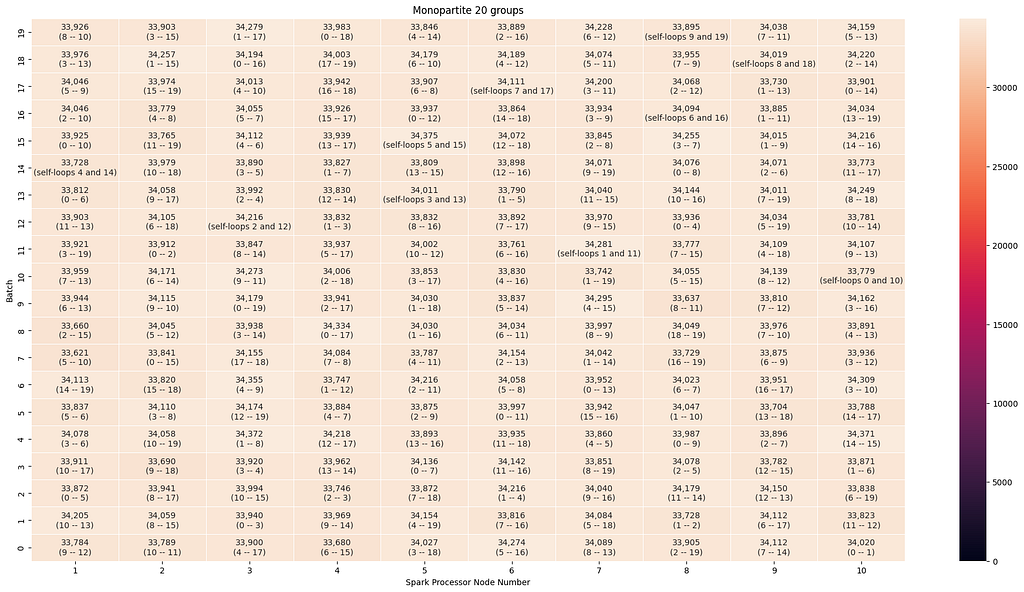
Monopartite
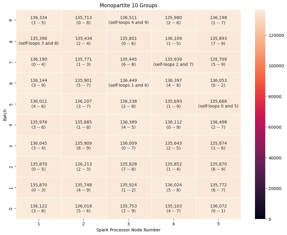
In some relationship datasets, the same node is the source node of some relationships and the target node of other relationships. For example, a DataFrame of phone call data might have columns for calling_number, receiving_number, start_datetime, and duration and require CALLED relationships between PhoneNumber nodes. The same PhoneNumber node can be the source for some CALLED relationships and the target for other CALLED relationships.
When running parallel_spark_loader.monopartite.group_and_batch_spark_dataframe(), the library uses the union of the source and target nodes as the basis for assigning nodes to groups. As with other scenarios, the number of groups that should be created is provided as an argument, and a greedy algorithm assigns node IDs to groups so that the combined number of source and target rows for the IDs in a group is roughly equal.
As with the other scenarios, the number of groups that the algorithm will assignis set with an argument. However, unlike the predefined components and bipartite scenarios, in the monopartite scenario, it is not recommended that the number of groups equals the number of executors in the Spark cluster. This is because a group can represent the source of a relationship and the target of a relationship. In the monopartite scenario, it is recommended to set num_groups = (2 * num_executors).
We can visualize the nodes within the same group as a single aggregated node and the relationships that connect nodes within the same group as a single aggregated relationship.
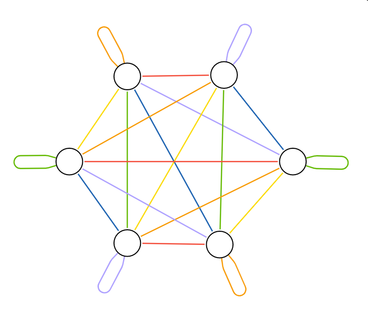
In the aggregated bipartite diagram, multiple relationships (each representing a group of individual relationships) connect to each node (representing a group of nodes). Because nodes could be either source or target, no arrowheads in the diagram represent relationship direction. However, the nodes are always stored with a direction in Neo4j. Using the rotational symmetry of the complete graph, the relationships are colored so that no relationships of the same color connect to the same node. The relationship colors represent the batches applied to the data.
In the diagram above, the relationship groups represented by red arrows can be processed in parallel because no node groups are connected to more than one red relationship group. After the red batch completes, each additional color batch can be processed in turn until all relationships have been loaded. Notice that with six node groups, each color batch contains three relationship groups. Self-loops on opposite sides of the hexagon are contained in a single group. This demonstrates why the number of groups should be larger than the number of Spark executors you want to keep occupied.
Benchmarking
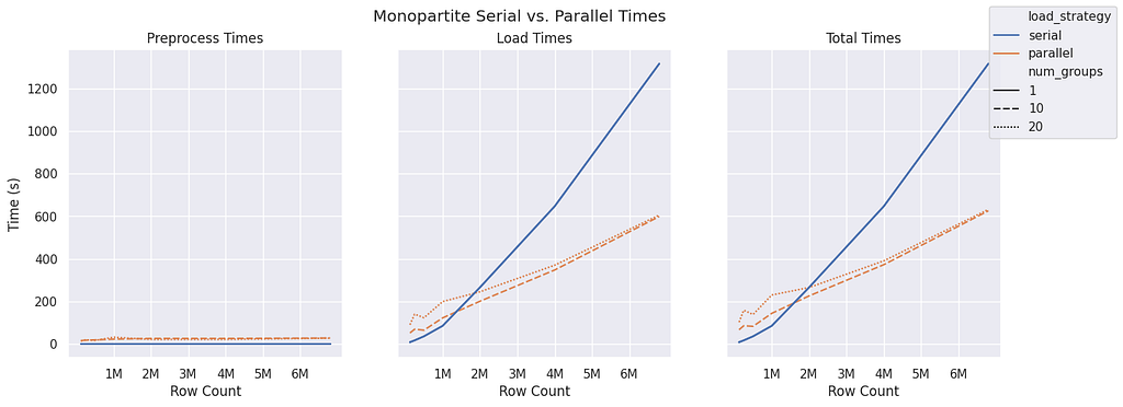
The necessary preprocessing steps to create groups and batches adds to the total time to complete ingestion, and adding multiple small transactions to the load increases transactional overhead for the Neo4j server. Therefore, using the Neo4j Parallel Spark Loader doesn’t improve the performance of loading small numbers of relationships over loading relationships serially. While improved performance occurs at different data sizes for different graph structures, the Neo4j Parallel Spark Loader package provides benefits only for large datasets. Generally, serial loading is recommended for jobs with less than 1 million rows. The benchmarking results are detailed below.
Datasets
Real datasets were used to evaluate each graph structure:
- Predefined components used data on Reddit threads.
- Bipartite used data on Amazon ratings.
- Monopartite used data from Twitch.
Methods
The benchmarking process was run in an Azure-hosted Databricks environment with the following configuration:
- Runtime → DBR 15.4 LTS Spark 3.5.0 • Scala 2.12
- Driver → Standard_D4ds_v5 • 16GB • 4 Cores
- Workers (5) → Standard_D4ds_v5 • 16GB • 4 Cores
For each graph structure (predefined components, bipartite, monopartite), preprocessing time and load time were measured for different data sizes and group numbers.
Each of the three graph structure methods were run with sample sizes of 125k, 250k, 500k, 1mil, 2mil, 4m rows, and the entire dataset. These sample sizes were randomly collected from the associated dataset.
Additionally, multiple group sizes were evaluated for each sample size. A group size of 1 was evaluated to evaluate serial performance. Two additional group sizes were selected for parallel evaluation:
- Predefined Components: 1, 5, 20
- Bipartite: 1, 5, 20
- Monopartite: 1, 10, 20
For each new sample size, a randomly selected set was obtained from the appropriate dataset. This same sample set was then used for each group size.
Performance was measured using a Neo4j Aura-hosted instance in an Azure environment with the following configuration:
- 24GB memory
- 48GB storage
- 5 CPU
Each relationship ingest query used MATCH to find the source and target nodes and CREATE to create the relationship. This was appropriate since the data contained no duplicate relationships.
After each ingestion run, the relationships were deleted from the database, and nodes were left to reduce the benchmarking runtime.
Both the Databricks instance and Aura instance were hosted in the same Azure region.
Overall Load Time Improvements
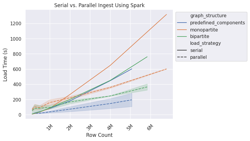
The chart above shows that the predefined components graph structure has improved load performance around the 250k row size, while bipartite and monopartite begin to show improvement around 1.5mil rows. The variance is from the different group sizes used for each graph structure. Serial ingest can only ever use one group, which is why there is no variance shown for that load strategy. Note that the preprocessing time is not accounted for in this chart and each dataset has a different size, so the largest row count for each graph structure varies.
Predefined Components
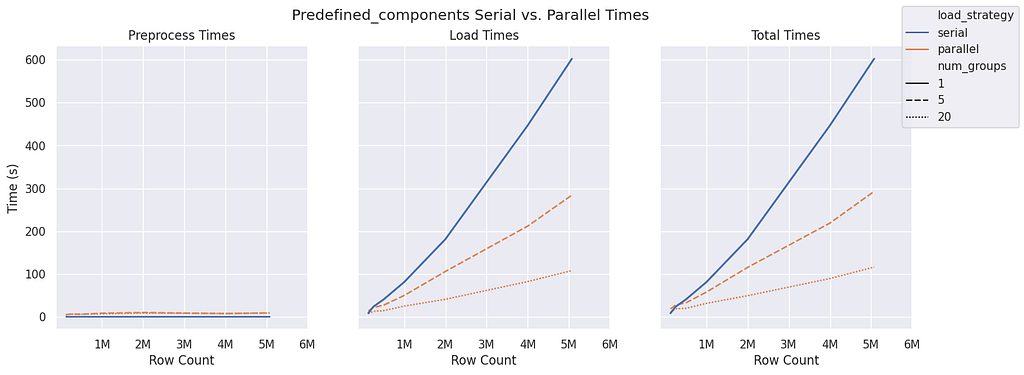
The predefined components graph structure requires very little preprocessing compared to bipartite and monopartite, and it remains fairly constant even as the sample size increases. There is also a significant improvement with more groups available during the ingestion phase. For load time alone, there appears to be nearly a 2x improvement between five and 20 groups once 2 million rows are reached. Due to the constant and minimal preprocessing time, this improvement is maintained when assessing the total time.
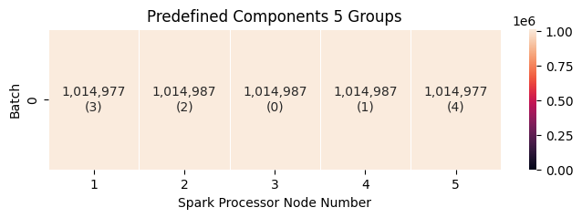
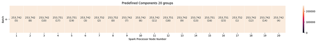
Predefined components always run in a single batch. For group sizes of five and 20, the groups are evenly distributed, which leads to efficient loading.
Bipartite
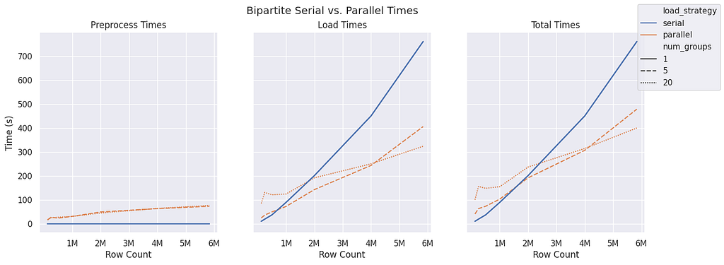
The bipartite graph structure sees preprocessing time begin to increase after about 1 million rows. Interestingly, for parallel ingest, a group size of five seems to be more performant than a group size of 20 until around 4 million rows. Both parallel group sizes don’t seem to match serial performance until a row count of 2 million is reached.
It’s important to note that the preprocessing time is higher here than in predefined components and monopartite because it has to group both the source nodes and target nodes individually.
Once again, the group sizes are evenly distributed, which leads to efficient loading in both groups of five and 20.
Monopartite
The monopartite graph structure seems to have similar performance with a smaller group size of 10 compared to 20 for all sample sizes. Both group sizes begin to outperform serial ingest near the 1.5 million row count.
The monopartite group sizes are evenly distributed, which leads to efficient loading in both group sizes of five and 20. Notice that for 10 groups, there are five executors, and for 20 groups, there are 10 executors. This is because a node can be both a source and a target.
Additional Improvements
Below are some additional ways to improve performance with the Neo4j Parallel Spark Loader Python Package.
CREATE Instead of MERGE
If there are no duplicated relationship rows in the DataFrame, it may be ingested using CREATE instead of MERGE in the relationship creation clause. This improves ingestion time by no longer performing a MATCH on the relationship to ensure that it doesn’t already exist before creating it. An example query:
MATCH (n:NodeA {id: "a"})
MATCH (m:NodeB {id: "b"})
CREATE (n)-[:HAS_RELATIONSHIP]->(m)
Property-Based Groups
The Neo4j Parallel Spark Loader will use count-based grouping during preprocessing. You may instead provide custom property-based groups to reduce preprocessing time.
A column named group must be created and passed to the batching function.
from pyspark.sql import DataFrame, SparkSession
from pyspark.sql.functions import expr

# all graph structures use the same ingest function
from neo4j_parallel_spark_loader import ingest_spark_dataframe

# we import the batching function from the bipartite module
# since our hypothetical data has a bipartite graph structure
from neo4j_parallel_spark_loader.bipartite import create_ingest_batches_from_groups

# init Spark
spark_session: SparkSession = (
    SparkSession.builder.appName("Workflow Example")
    .config(
        "spark.jars.packages",
        "org.neo4j:neo4j-connector-apache-spark_2.12:5.1.0_for_spark_3",
    )
    .config("neo4j.url", "neo4j://localhost:7687")
    .config("neo4j.authentication.type", "basic")
    .config("neo4j.authentication.basic.username", "neo4j")
    .config("neo4j.authentication.basic.password", "password")
    .getOrCreate()
)

# load the DataFrame
sdf: DataFrame = spark_session.createDataFrame(data=...)

source_key = "customer_id"
target_key = "store_id"

# create source and target columns
rel_df = rel_df.withColumn('source_group',
           expr(f"cast(right({source_key}, 2) as int) % 20"))
rel_df = rel_df.withColumn('target_group',
           expr(f"cast(right({target_key}, 2) as int) % 20"))

# create the final group column to be used during ingest
rel_df = rel_df.withColumn("group",
           expr("cast(source_group as string) || '_' || cast(target_group as string)"))

# use the groups defined above to create batches
batch_rel_df = create_ingest_batches_from_groups(rel_df)

query = """
MATCH (o:Order {id: event['order_id']}),
(p:Product {id: event['product_id']})
MERGE (o)-[r:INCLUDES_PRODUCT]->(p)
ON CREATE SET r.quantity = event['quantity']
"""

# load data into Neo4j
ingest_spark_dataframe(batch_rel_df, "Overwrite", {"query": query})
Pass Group Number to Ingest Function
You may pass the num_groups argument to the ingest_spark_dataframe() function. This removes the need to find the number of groups in the function and reduces processing time.
The num_groups argument here should match the num_groups argument used during grouping and batching.
from pyspark.sql import DataFrame, SparkSession

from neo4j_parallel_spark_loader import ingest_spark_dataframe
from neo4j_parallel_spark_loader.bipartite import group_and_batch_spark_dataframe

spark_session: SparkSession = (
    SparkSession.builder.appName("Workflow Example")
    .config(
        "spark.jars.packages",
        "org.neo4j:neo4j-connector-apache-spark_2.12:5.1.0_for_spark_3",
    )
    .config("neo4j.url", "neo4j://localhost:7687")
    .config("neo4j.authentication.type", "basic")
    .config("neo4j.authentication.basic.username", "neo4j")
    .config("neo4j.authentication.basic.password", "password")
    .getOrCreate()
)

purchase_df: DataFrame = spark_session.createDataFrame(data=...)

NUM_GROUPS = 8

# Create batches and groups
batched_purchase_df = group_and_batch_spark_dataframe(
    purchase_df, "customer_id", "store_id", NUM_GROUPS
)

# Load to Neo4j
includes_product_query = """
MATCH (o:Order {id: event['order_id']}),
(p:Product {id: event['product_id']})
MERGE (o)-[r:INCLUDES_PRODUCT]->(p)
ON CREATE SET r.quantity = event['quantity']
"""
ingest_spark_dataframe(
    spark_dataframe=batched_purchase_df,
    save_mode= "Overwrite",
    options={"query":includes_product_query},
    # pass the optional num_groups arg here
    num_groups=NUM_GROUPS
)
Summary
The Neo4j Parallel Spark Loader Python package provides useful tools for those looking to improve large-scale ingestion jobs. This package alleviates the headaches caused by loading relationships in parallel by appropriately grouping and batching the data before ingestion. This leads to decreased load times and decreased total ingestion times at high data volumes.
To learn more, check out the Neo4j Connector for Apache Spark docs.
Use Neo4j Parallel Spark Loader to Improve Large-Scale Ingestion Jobs was originally published in Neo4j Developer Blog on Medium, where people are continuing the conversation by highlighting and responding to this story.
Share Article


Explore
Related Articles
Text2Cypher Across Languages: Evaluating Foundational Models Beyond English