Bolster Your Cybersecurity by Visualizing Attack Graphs With Neo4j & G.V()

From malware crypto-mining attacks to ransomware gangs, the goal of a cyberattack is often the same as any heist: find the shortest possible path to the valuables and get out quickly. It’s all about route finding, and that’s why it’s long been known that cyber-attackers frequently visualize their targets as graph networks, also known as attack graphs.

To protect your own system, defenders need to think the way an attacker does. For example, Wiz recently discovered vulnerabilities in an Ingress NGINX controller using an attacker mindset.

Even if your system only uses a regular relational database for day-to-day operations, your cybersecurity team needs a way to foresee the most likely potential attack paths and react quickly. For complex interconnected systems, graph database technology — and the graph visualization and analysis to accompany it — are critical tools for identifying cyberattack risks.

Fortunately, a Neo4j instance is the perfect environment to conduct this kind of cybersecurity analysis. You can even couple your Neo4j instance with a graph visualization tool like G.V() — this will help you quickly and easily identify vulnerabilities in your system with minimal query writing. If you use G.V()’s Graph Data Explorer, you may not need to write any code at all.

Let’s take a closer look.

Thinking Like an Attacker

An attacker starts by gaining access to your system anywhere they can. Once inside, they’ll try to progress through your network.

The attacker often doesn’t know the structure of your network in advance, so they’ll usually proceed with a toolbox of versatile techniques and a see-what-works approach. They’ll rarely find what they’re looking for immediately. Instead, they’ll explore your network, hopping from location to location.

Anything an attacker successfully gains access to is a resource — this could be access to a new location, a new piece of code, log-in credentials, or just useful information, such as the location of another resource. Any technique an attacker uses to get from one resource to another is an attack.

The goal is to find something valuable — something we’ll call a critical asset. A critical asset is a deliberately vague concept that could be a number of things, but the important thing to know is that it’s something the attacker wants and the defender can’t afford to lose. For example, a critical asset might be a resource that gives the attacker full control over the system.

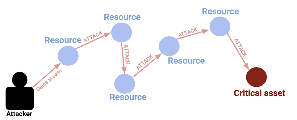
You can see right away why hackers tend to visualize computer networks as graphs. An attacker probably isn’t interested in understanding every part of your system or viewing every resource. Rather, an attacker cares about finding a viable path to the critical asset through all the other resources. Picturing the system as a graph helps them find and conceptualize those paths quickly.

This is an attack graph.

In pseudo-Cypher, we can represent attack graphs how you might expect — we use (⬤ Resource) and (⬤ Critical asset) nodes to represent each entity. We represent any hypothetical movement an attacker might make between two nodes as [ATTACK] relationships.

A good graph model of the system — when coupled with good data visualization and analysis — gives defenders an advantage over attackers. Remember, attackers don’t usually know the layout of the system in advance, but defenders do!

Modeling a Kubernetes Cluster

In practice, a network will contain many kinds of resource and critical asset nodes. They likely will have their own properties, and this will affect the types of attack paths that are possible.

For this discussion, we’ve chosen to use a sample dataset illustrating a Kubernetes cluster, and we adopt the KubeHound description of that cluster.

Here are the kinds of nodes that exist in our example system:

• (⬤ Volume) — A location where persistent memory is stored within the cluster
• (⬤ Node)* — A worker machine within the Kubernetes cluster that runs pods
• (⬤ Pod) — A deployable unit within a node that runs one or more containers
• (⬤ Container) — A small environment containing an application
• (⬤ PermissionSet) — A set of actions allowed by a given user/identity, and the only critical asset node in the system
• (⬤ Identity) — A user or service account awarded upon authentication
• (⬤ Endpoint) — A connection point for a pod

Note: The term “node” means both “an entity in a graph” and “a worker machine in a cluster,” so I’ll clarify which type of node I mean by using “node” to refer to the former and (⬤ Node) for the latter.

Here’s a greatly simplified version of the data model showing some sample attack types. Some are simple, some highly abstract. For example, one can image the generic idea that an attacker may be able to gain access to your system via an exposed endpoint. We represent that concept by the [ENDPOINT_EXPLOIT] attack, without worrying too much about the mechanism. Others attacks, like [TOKEN_STEAL], describe an attack that is more specific: stealing a mounted service account token.

Of course, there are many more possible types of cyberattack than are shown here. Understanding individual attack types will be important later, when interpreting and responding to your cybersecurity graph. That’s what will let you address the vulnerabilities you discover in your system.

But for now, we’re just focused on identifying dangerous paths, so we won’t worry too much about classifying the different kinds. All we need to know is that multiple relationship types exist.

Download the Sample Dataset

Now that we understand the data model, we’ll manage our example security cluster in Neo4j. We’ll also walk you through how to visualize it in G.V().

Everything here is something you can do yourself. The sample dataset is available in ZIP form on GitHub and can be used inside a Neo4j Sandbox. You can upload the data directly via the data importer. Just select Open model (with data) in a Neo4j Sandbox and select the ZIP file. We’ve also included the raw data in CSV form.

If you haven’t already installed G.V(), head on over to the download portal, since you’ll need it to follow along.

Once you have G.V() downloaded and open, click New Database Connection.

From there, you just need to select Neo4j as your Graph Database Type and enter your Bolt address and port. Once you do this, you’ll be prompted for your username and password.

Enter your details and submit your connection — it’s as easy as that!

Graph Visualization With G.V()

To save us a lot of time, let me introduce you to G.V()’s new Graph Data Explorer. Traditionally, if you wanted to see all the data in your graph database, you’d have to run a Cypher query. Something like:

MATCH p=()-[]-() RETURN p LIMIT 10000

While G.V() is fully Cypher-compatible, and you absolutely can run this from the query editor if you like, the Graph Data Explorer eliminates the need to construct code-based queries like this for intuitive data exploration. In fact, we’re about to do some cybersecurity analysis without coding at all. But we’ll include the Cypher commands in any case — just in case you prefer to follow along that way.

Let’s try looking for any node connected to another node in our graph.

Now we have a general overview of the situation. All the attack paths in our system are visible at once, and we can use the force-directed layout to get a good overview of the relationships between nodes, or the community layout to see what kinds of resources are present in our system.

Since (⬤ Endpoint) graph nodes are among the most common points of entry for an attack, we’ve highlighted these and turned off labels for all other nodes. This lets you see at a glance where attacks from an exposed endpoint might begin.

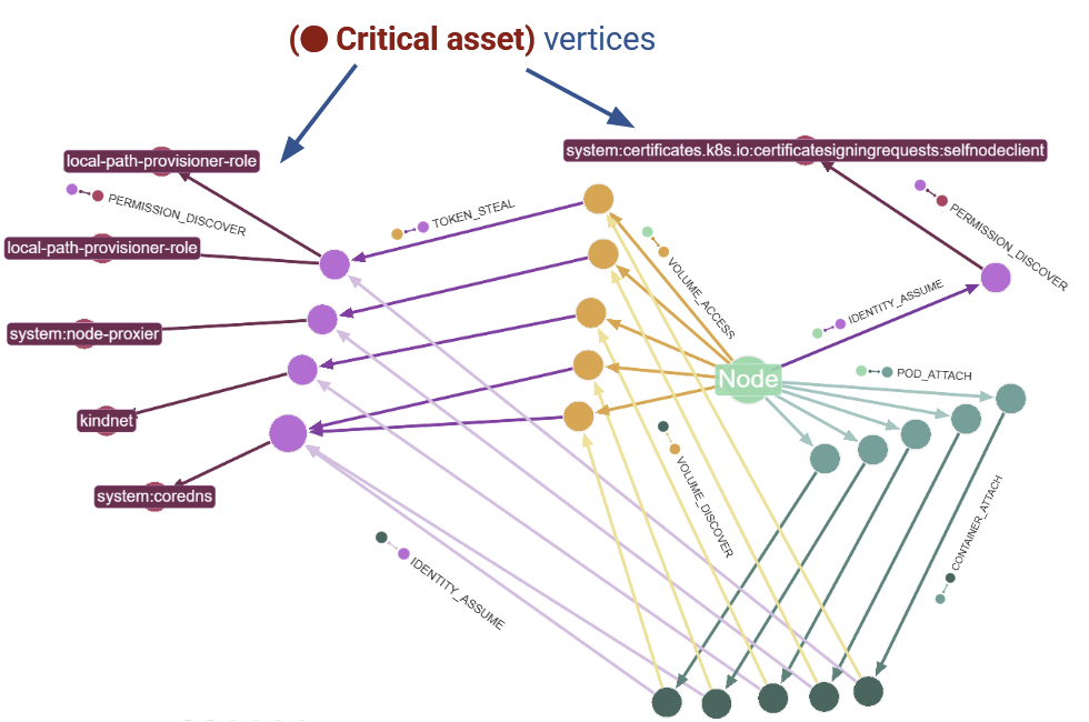
If there are particular graph nodes or relationships you want to investigate for vulnerabilities, it’s as easy as a few clicks to highlight the node of interest. Let’s take a look at the worker machine (⬤ Node) with the name kubehound.test.local-control-plane.

We can see all the different types of attacks that can be made in and out of this worker machine (⬤ Node).

This graph visualization above lets us draw a mental picture of this resource:

• Many targets — There are a large number of (⬤ Volume) and (⬤ Pod) resources directly accessible if the attacker performs a successful [VOLUME_ACCESS] or [POD_ATTACH] attack.
• Exposed identity — There is an adjacent (⬤ Identity) resource vulnerable to [IDENTITY_ASSUME] attack.
• Container threat — There is one relationship leading into the resource. An attacker could gain access to this node resource from an adjacent (⬤ Container) graph node using a [CE_PRIV_MOUNT] attack.

It’s also easy to modify our graph further to reflect the security measures as we implement them.

For example, let’s say we’ve done a lot of work protecting our volumes, so they’re less vulnerable to volume access attacks. Since we’re less worried about these kinds of attacks now, we’d like to focus on other areas.

We have two options for doing this. The first is to toggle off the [VOLUME_ACCESS] relationships. This keeps the volume nodes visible, so we can ensure that no other types of attacks are coming to or from those resources.

If — and only if — we’re confident that the volume resources are now effectively isolated from our worker machine (⬤ Node) resource, we can just toggle off the (⬤ Volume) nodes completely. This lets us focus entirely on other resources.

But what about critical assets?

Recall that all our critical assets are of the type (⬤ PermissionSet). As we can see, there are none among our worker machine (⬤ Node)’s closest neighbors. But, if we allow multiple hops, there could still be a way to reach a critical asset via more distant neighbors. We’d like to see if such paths exist.

Let’s say we’d like to check if our worker machine (⬤ Node) connects to any critical assets in 10 or fewer hops:

MATCH path = (start {name: ‘kubehound.test.local-control-plane’}) →{1,10}(end)
WHERE (end.critical=True
AND ALL(n IN NODES(path)[1..] WHERE n <> start))
RETURN path

We can see there are several viable paths leading out of our resource that leave multiple critical assets exposed! Each path shown here represents a hypothetical risk to our system.

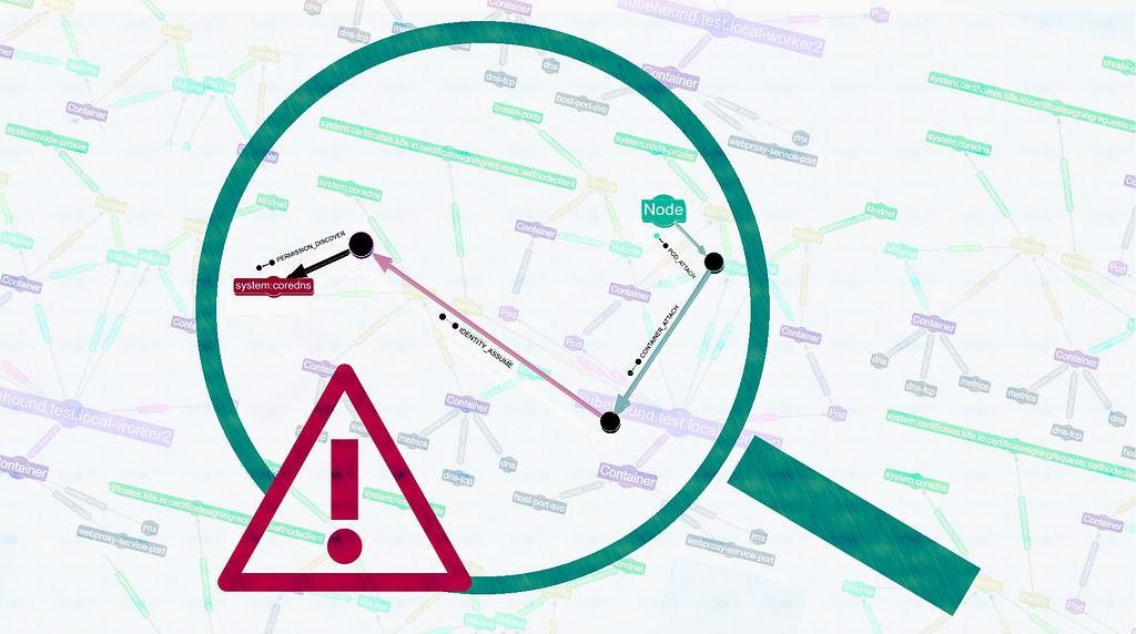
Let’s highlight just one attack path.

Since the system:coredns (⬤ PermissionSet) is a critical asset, let’s focus on this node in particular. Instead of looking at paths from our starting resource — the (⬤ Node), which we selected somewhat randomly — we instead want to understand how vulnerable this critical asset is in general.

Attackers typically begin their attack from an endpoint, so let’s look for relationships that could expose this asset to endpoints.

We can reverse our previous query to see all the (⬤ Endpoint) connections from this asset:

MATCH path = (start:PermissionSet {role: ‘system:coredns’}) — {1,10}(end)
where (end.label=’Endpoint’ AND ALL(n IN NODES(path)[1..] WHERE n <> start))
RETURN path

We can see right away that we actually don’t need to worry too much about the kubehound.test.local-control-plane (⬤ Node) if we’re analyzing attacks from endpoints, since there aren’t any paths connecting that graph node to an endpoint path. We can see, however, that there are some containers, volumes and identity nodes that we might care about.

For a more general overview of our system, we could see all paths that link an endpoint to any critical asset in fewer than ten hops:

MATCH path = (start:Endpoint) →{1,10}(end:PermissionSet)
WHERE (end.critical=true
AND ALL(n IN nodes(path) WHERE size([m IN nodes(path) WHERE m = n]) = 1))
RETURN DISTINCT path LIMIT 1000

We can see that there are two (separate) categories of attack path:

• Category #1: An attacker can proceed through either of the coredns (⬤ Container) nodes.
• Category #2: An attacker can proceed through the worker machine (⬤ Node), kubehound.text.local-worker2.

Even though categories 1 and 2 both contain a number of sub-paths, we can greatly strengthen our security system and cut off most attack paths by focusing on choke points like this.

By focusing their energy on the paths that really matter, defenders ensure maximum security in the system. This is a task graph visualization is uniquely suited for. Robust attack graphs enable identification of vulnerabilities at a glance, giving defenders the insights and time they need to shore up their defenses.

Summary

You’ve now experienced a taste of just how powerful graph visualization can be in the world of cybersecurity. But this is just the beginning: Neo4j with G.V() is a powerful combination that provides deep insight into your system strengths and vulnerabilities from every angle and scale.

Cyberattacks always follow rules, no matter how sophisticated they are, and that makes them predictable. With a robust graph data model and a diligent cybersecurity team, there’s no attack path you won’t see coming.

Resources

• What Is a Graph Database?
• Visualize your data in Neo4j
• Neo4j Cypher Query Language

---

How to Bolster Your Cybersecurity by Visualizing Attack Graphs With Neo4j and G.V() was originally published in Neo4j Developer Blog on Medium, where people are continuing the conversation by highlighting and responding to this story.