Cypher and the Cipher Manuscript

Predicting the Voynich Manuscript’s Provenance With Neo4j and Graph Data Science

TL;DR: This article provides a walkthrough, using Neo4j‘s link prediction feature to predict potential previous owners of the Voynich Manuscript. It then explores one promising candidate, Hartmann Schedel, in more detail.

The Voynich Manuscript has been the subject of academic research, fringe conspiracy, and everything in between.

Written in a dead language, lost script, or keyless cipher — all three or none — so far, it remains uncracked. From NSA and Bletchley Park cryptographers to unassuming historians and lone researchers, it’s ensnared countless curious victims. So many debunked solutions exist, and one Beinecke Rare Book & Manuscript Library librarian described the Voynich as “the place where academic careers go to die.” Since its supposed creation in the 15th century, only one truth persists: You don’t crack the Voynich — it cracks you.

If you’re not already familiar with the manuscript, you can view each page in eye-splitting detail. For a rundown of the available research, check out voynich.nu. You can even query the manuscript on voynichese.com.

Many attempts have been made to decode the manuscript using statistical, machine learning, and AI techniques. In fact, Voynich Attacks is an active forum dedicated solely to computational attacks on the manuscript.

In this article, we’ll look at another ML approach available to us: ML link prediction in Neo4j. However, we won’t attempt to decode the manuscript, for that’s where madness lies. Instead, we’ll use Neo4j’s link prediction feature to predict plausible previous owners.

The Voynich Manuscript’s Provenance

There are two main gaps in the Voynich Manuscript’s provenance.

Emperor Rudolf II is generally accepted as the earliest known owner of the manuscript. There is evidence to suggest that he acquired the manuscript from Karl Widemann, a German physician, who may in turn have inherited it from Leonhard Rauwolf, a botanist. Other theories suggest that Rudolf acquired it from John Dee, court astronomer to Elizabeth I, occultist, Hermetic philosopher, and all-around kooky cat. Regardless, Rudolf allegedly then passed it on to Jakub Hořčický (also known as Jacobus Horcicky), his personal physician.

The next known owner, Jiří Bareš (also known as Georg Baresch), was a Bohemian alchemist. When Baresch died, the manuscript was inherited by the rector of Charles University in Prague, Jan Marek Marci. Marci sent it to Athanasius Kircher, a Jesuit scholar at the Collegio Romano, whom he believed to be the only person capable of deciphering the text. There it remained until it was discovered and purchased from the College by Wilfred Voynich in 1912. Currently, it resides in the Beinecke Rare Book & Manuscript Library at Yale University.

Importing Manuscript Data to a Neo4j Graph

“If only we had access to a dataset of provenance data for thousands of medieval manuscripts,” I thought, “we could use link prediction to infer likely owners.” Not only do we have access to such a dataset but it’s already structured as a graph.

Meet Mapping Manuscript Migrations, an aggregated database of linked collections of The Schoenberg Institute for Manuscript Studies, the Bodleian Libraries and the Institute for Research and History of Texts.

The online platform allows users to engage with manuscript metadata through various lenses — however, the entire knowledge graph is available for download.

Using Neosemantics, we can import the dataset directly into a fresh Neo4j database.

The underlying data model used for Mapping Manuscript Migrations is highly complex, and an explanation lies outside the scope of this article. However, the nodes of most concern are:

• F4_Manifestation_Singleton — The actual physical manuscript
• E21_Person — An actual physical person

Manuscripts connect to Person nodes via:

-[:P51_has_former_or_current_owner]->

To learn about the data model in more detail, see the Mapping Manuscript Migrations documentation, FRBRoo documentation, and CIDOC CRM documentation. If you’d like to learn more about data modeling in a Neo4j graph database, check out Graph Data Modeling Fundamentals at GraphAcademy.

What is Link Prediction?

Link prediction is a common ML task applied to graphs: training a model to infer where relationships could exist.

In this section, I’ll run through the exact steps I used to run link prediction on the manuscript in Neo4j. If you want to download the dataset above and follow along, you can. If you’re more interested in the results, feel free to skip this section.

The high-level steps:

1. Train an embedding model
2. Run the embedding model
3. Train the link prediction model
4. Run the link prediction model

Let’s get started.

Adding Node Embeddings

If you’re not sure what embeddings are, check out this Wiki on word embeddings.

Node embeddings are similar, except, instead of representing the semantic similarity between words, they represent the topological similarity between nodes in a graph, based on their relationships to other nodes in that graph.

There are many ways to skin a node embedding, and the following method isn’t necessarily the best — it’s just what we’re doing for this article.

Step 1: Project the Graph

When running anything in Neo4j Graph Data Science, we always project a subgraph first, manipulate that projected graph, then write any changes we want to keep back to the main graph. So, we’ll project the following subgraph; it includes only those nodes between which we intend to predict links:

MATCH (source)
WHERE NOT source:Database AND NOT source:Dataset
OPTIONAL MATCH (source)-[r]->(target)
WHERE NOT target:Database AND NOT target:Dataset
WITH gds.graph.project(
'voynich-graph',
source,
target,
{
  sourceNodeLabels: labels(source)[0],
  targetNodeLabels: labels(target)[0],
  relationshipType: type(r)
},
{
  undirectedRelationshipTypes: ['*']
}
) AS g
RETURN
  g.graphName AS graph,
  g.nodeCount AS nodes,
  g.relationshipCount AS rels,
  g.projectMillis AS timeInMs

The resulting projection includes every single node and relationship type except for Database and Dataset nodes — they connect to everything else, which could skew our results.

Step 2: Train a GraphSAGE Model

With GraphSAGE, you first train a custom node embedding model. Afterward, you can run that model on your projection to get node embeddings.

Before training the model, we add some properties to our graph projection. Our model can then use these properties as clues. For the purposes of this article, we’ll just add degree centrality, which helps us find popular nodes in the graph based on the number of relationships each node has.

CALL gds.degree.mutate(
'graph-sage',
  {
    mutateProperty: 'degree'
  }
) YIELD nodePropertiesWritten

Using mutate, we don’t actually save this output to the main graph. Instead, they’re only added to our graph projection and disappear when we drop the projection.

Step 3: Sample a Subgraph

Our current graph is huge — millions of nodes. If we tried to train GraphSAGE on it, we’d have to wait hours for it to finish. Instead, let’s get a small sample of the graph using random walk with restarts sampling:

CALL gds.graph.sample.rwr(
'voynich-graph-sample',
'voynich-graph',
  {
    samplingRatio: 0.05,
    restartProbability: 0.1,
    nodeLabelStratification: true,
    concurrency: 1,
    randomSeed: 42
  }
)

Now, if we train our GraphSAGE model on this sample, it will still run on the larger graph, but it won’t take hours to finish training. Once this sample finishes, we’re left with 192,000 nodes and 745,000 relationships.

Step 4: Train the Embedding Model

To train the embedding model, we enter this into the Neo4j Browser:

CALL gds.beta.graphSage.train(
  'voynich-graph-sample',
  {
    modelName: 'voynichEmbeddings',
    featureProperties: ['degree'],
    maxIterations: 15,
    learningRate: 0.01,
    epochs: 6,
    batchSize: 200,
    searchDepth: 5,
    randomSeed: 42
  }
)

The following chart shows the training loss after the model has seen the data six times.

You could think of the downward trend as how much better the model gets each time it goes through the data. When that trend curve flattens out, it’s time to stop. If it goes flat for a long time, we’ve probably gone too far. If it starts going up, there are likely more than a few problems with our data and/or our configuration.

In this case, our model hasn’t yet finished getting any better, so we may have stopped too early. It is, however, close enough for testing.

Step 5: Run the Embedding Model

Finally, we run our model to get node embeddings:

CALL gds.beta.graphSage.mutate(
'voynich-graph',
{
  mutateProperty: 'voynich_embeddings',
  modelName: 'voynichEmbeddings'
}
) YIELD nodeCount, nodePropertiesWritten

On the Mapping Manuscripts Migrations graph, this embedding pass produces almost 4 million embeddings in only 2 minutes and 17 seconds.

Now that we have some embeddings, let’s build our link prediction pipeline.

Build a Link Prediction Pipeline

There are a number of steps to building your link prediction pipeline. We’ll run through what I did step by step.

Step 1: Call the Pipeline Into Existence

The command below calls Graph Data Science and tells it to create a pipeline called voynich-pipe:

CALL gds.beta.pipeline.linkPrediction.create('voynich-pipe')

Step 2: Add Link Features

Next, we add link features to our pipeline, so the model can use them as part of its training. Link features can be any of the properties that exist in your graph projection.

In our case, we have degree centrality and embeddings from our GraphSAGE model. We can add these via three similarity functions:

• Cosine
• Hadamard
• L2

With GDS link prediction, you can choose to use all three if you like. If you’re following along, don’t worry too much about what these mean or do. Just remember:

• They are different methods of calculating similarity between two nodes.
• You can add node properties to them as clues.
• You have to use at least one, but you can use up to all three.

I only included Hadamard and Cosine:

CALL gds.beta.pipeline.linkPrediction.addFeature('voynich-pipe','HADAMARD', {
  nodeProperties: ['sage_embeddings', 'degree']
})

CALL gds.beta.pipeline.linkPrediction.addFeature('voynich-pipe','COSINE', {
  nodeProperties: ['voynich_embeddings', 'degree']
})

Step 3: Configure Your Train/Test Split

Next, we configure our train/test split. The way the model learns is functionally not so different from us. It needs material to learn from and material to check its understanding. By splitting the graph into train/test segments, we can:

• Show the model one section of the graph, from which it learns
• Test it on another, smaller section of the graph, which tells it how well it understands the graph

CALL gds.beta.pipeline.linkPrediction.configureSplit('voynich-pipe', {
  testFraction: 0.2,
  trainFraction: 0.6,
  validationFolds: 3,
  negativeSamplingRatio: 1.0
})

Step 4: Add Candidate Models for Training

Finally, we add candidate models to our pipeline. In Graph Data Science link prediction, there are three potential model types you can train:

1. Logistic regression
2. Random forest
3. Multilayer perceptron

The finer details of each model don’t really matter for us. If we add all three to our pipeline, Graph Data Science will train them all and choose the best-performing model.

CALL gds.beta.pipeline.linkPrediction.addLogisticRegression('voynich-pipe', {
  maxEpochs: 100,
  penalty: 0.5
})
YIELD parameterSpace
RETURN parameterSpace

CALL gds.beta.pipeline.linkPrediction.addRandomForest('voynich-pipe', {
  numberOfDecisionTrees: 100,
  maxDepth: 10
})
YIELD parameterSpace
RETURN parameterSpace

CALL gds.alpha.pipeline.linkPrediction.addMLP('voynich-pipe', {
  hiddenLayerSizes: [128, 64],
  maxEpochs: 100,
  patience: 2
})
YIELD parameterSpace
RETURN parameterSpace

Step 5: Train Your Model

Next, we train our model and wait. In the example below, I specified that this model should only try to predict links between F4_Manifestation_Singleton nodes and E21_Person nodes:

CALL gds.beta.pipeline.linkPrediction.train('voynich-graph', {
  pipeline: 'voynich-pipe',
  modelName: 'voynich-provenance',
  sourceNodeLabel: 'F4_Manifestation_Singleton',
  targetNodeLabel: 'E21_Person',
  targetRelationshipType: 'P51_has_former_or_current_owner',
  metrics: ['AUCPR'],
  randomSeed: 42
}) YIELD modelInfo, modelSelectionStats
RETURN
  modelInfo.bestParameters AS winningModel,
  modelInfo.metrics.AUCPR.train.avg AS avgTrainScore,
  modelInfo.metrics.AUCPR.outerTrain AS outerTrainScore,
  modelInfo.metrics.AUCPR.test AS testScore,
  [candidate IN modelSelectionStats.modelCandidates | 
    candidate.metrics.AUCPR.validation.avg] 
      AS validationScore

Finally, we get our model. In this run, random forest was the best performer — the other two were discarded.

The average train score for our model comes out to be 0.96 out of a potential 1. Essentially, that means that when the model was tested on our held-out set of links, it was correct 96 out of 100 times on average. Suspiciously good! The performance of models in captivity rarely match those same models out in the wild, so let’s test it.

Step 6: Run Your Link Prediction Model

Next, we simply call the model on our projected graph:

// Approximate search
CALL gds.beta.pipeline.linkPrediction.predict.mutate('voynich-graph', {
  modelName: 'voynich-provenance',
  sourceNodeLabel: 'F4_Manifestation_Singleton',
  targetNodeLabel: 'E21_Person',
  relationshipTypes: ['P51_has_former_or_current_owner'],
  mutateRelationshipType: 'APPROX_PREDICT_P51_OWNER',
  mutateProperty: 'probability',
  topK: 10,
  sampleRate: 0.5,
  randomJoins: 10,
  maxIterations: 100,
  concurrency: 1,
  randomSeed: 42
})
YIELD relationshipsWritten, samplingStats

Step 7: Write Relationships Back to the Main Graph

Finally, we can write these relationships back to the graph:

CALL gds.graph.relationship.write(
  'voynich-graph',
  'APPROX_PREDICT_P51_OWNER',
  'probability'
)
YIELD graphName, 
      relationshipType, 
      relationshipProperty, 
      relationshipsWritten, 
      propertiesWritten

Now, to see which new links have been predicted for the Voynich Manuscript, we just need the following query:

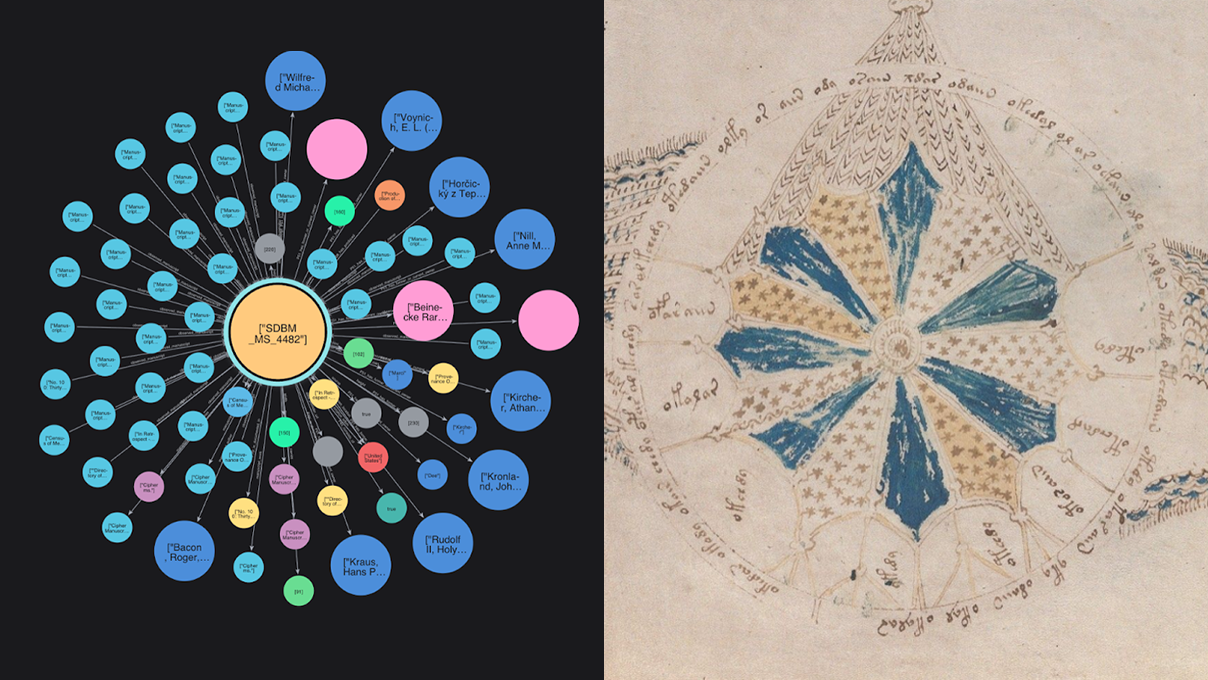
MATCH 
  (vm:F4_Manifestation_Singleton 
    {uri:'http://ldf.fi/mmm/manifestation_singleton/sdbm_4482'}
      )-[r:APPROX_PREDICT_P51_OWNER|P51_has_former_or_current_owner]->(k)
RETURN vm, r, k

Interpreting the Results

Running our prediction model on the graph returns these predictions:

The yellow links are those existing links from the Mapping Manuscript Migrations dataset; the blue links are those that the model predicts to be potential previous owners:

At this point, we should temper our expectations. We’re highly unlikely to find a magic link to a previous owner of the Voynich Manuscript — they may not even be in this database.

There are some great candidates here, and some who simply don’t make sense. However, just for fun, let’s test the plausibility of one particularly interesting candidate: Hartmann Schedel.

Hartmann Schedel: A Plausible Candidate

Hartmann Schedel was a German physician, historian, and cartographer. Lesser known, he was a student of alchemy and Hermetic mysticism. He compiled and edited the text to the Nuremberg Chronicle, one of the most popular early printed books anywhere in the world, in the 15th century. Let’s see if we can string some plausible threads from the Voynich to Schedel.

Connection 1: Northern Italian Medicine

Many consider the Voynich Manuscript to be some kind of encoded medicinal text. Some of the earliest guesses as to the location of its creation point toward Northern Italy — although that’s far from certain.

Hartmann received his doctorate from the University of Padua in 1466, following in the footsteps of his older cousin, Hermann, who held a doctorate from the same university. Throughout a series of letters, Hermann asks Hartmann to acquire various manuscripts for him, and Hartmann does his best to comply. Both Hermann and Hartmann are in the right place (maybe) at the right time (definitely).

Connection 2: Bibliophagus

Hartmann was a voracious reader, copyist, and one of the world’s most prolific manuscript collectors. In one letter to Hermann, he refers to himself as a bibliophagus or “book-eater.” By the time of his death in 1514, Hartmann’s collection contained hundreds of manuscripts — many of which he’d copied himself by hand.

There are at least two-and-a-half surviving indexes of Schedel’s extensive library collection. I qualify the half because one of them is essentially a scrapbook of random scribbles and scrawls, afterthought notes, and sections of torn-out pages.

They contained books on a broad array of topics — from medicine, law, and poetry to alchemy, astrology, witchcraft, and hermeticism. While many of these books have Voynich-adjacent descriptions, I checked and none of the descriptions precisely describe the text in any recognizable way. That said, according to Bettina Wagner, there must be at least one other lost inventory of Schedel’s library. Given that the Munich and Berlin versions don’t perfectly match in their inventories, one might reasonably expect the third version to differ, too. Schedel is as likely as anyone to have owned an obscure, impenetrable manuscript.

Connection 3: Hebrew and Hermetic Mysticism

According to Ilona Steinmann, Schedel’s book index did not faithfully list every single foreign language title.

There is one particularly telling entry: ‘The finest and most beautiful library, collected with the greatest eagerness and care, adorned with Greek, Latin, Hebrew, and foreign authors.” This section doesn’t list said foreign texts but treats them as a group. As Steinmann points out, Schedel couldn’t read Hebrew — but that didn’t stop him from collecting Hebrew texts by various means. If Hartmann had owned the Voynich, he would likely have included it here.

We’re now officially aboard the Dan Brown Express, hurtling toward intellectual doom — so let’s keep going.

Connection 4: The “Lost” Book

According to this letter, Hartmann had sent a damaged book to a Brother Nonnosus of Michaelsberg Abbey in Bamberg. It had been covered in pitch, leaving the pages bound together. Hartmann had hoped Nonnosus would be able to separate the leaves and restore the text. According to the letter, Nonnosus dared not try for fear of damaging it further. Nonnosus describes the text as “illegible.”

Nonnosus’ colleague, Eberhard, judged that the parchment appeared new and the writing recent and very thin. He thought it most likely a “useless or false book,” intended to trick Christians into thinking it contained secrets or antiquities. The description rhymes with the Voynich. For various reasons, however — not least its state of disrepair — this likely isn’t it.

Connection 5: Augsburg

Stefan Guzy has found relatively compelling evidence that Karl Widemann was the previous owner of the Voynich Manuscript, before Rudolf II. Widemann was an Augsburgian physician and alchemist. He may have inherited the text from Leonhard Rauwolf, another Augsburgian physician.

Hartmann Schedel is not without direct connections to Augsburg:

• According to an essay by Walter Bauernfeind, Heinrich Schedel, Hartmann’s paternal uncle, relocated to Augsburg in 1433.
• Hermann, his cousin, had been working as a physician and leading humanist in Augsburg at the very time that Hartmann had been sending him manuscripts from Italy.
• In 1552, Hartmann Schedel’s grandson, Melchior, sold 371 manuscripts from Hartmann’s library to Johann Jakob Fugger, member of a wealthy banking family in Augsburg.
• Hartmann’s greatest work, the Nuremberg Chronicle, was pirated by an Augsburgian printer.

If Schedel had been in possession of the manuscript, there’s more than one plausible path for it to reach Augsburg.

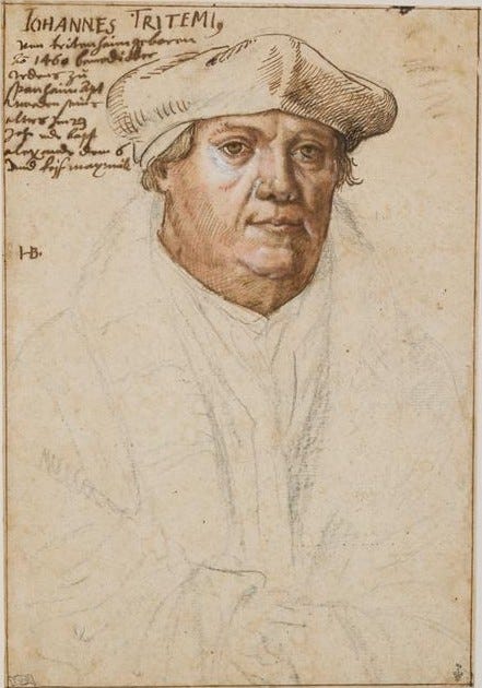
Connection 6: Trithemius

Trithemius is often cited among potential candidates as an author of the Voynich Manuscript. Known as the founder of modern cryptography, he wrote two works on the subject.

Steganographia, the more famous of the two, appears at first to be a magical text about using spirits to communicate over long distances. However, it’s actually a cryptographic text masquerading as an occult instruction manual. For some, it’s both. Regardless, at the time of its publication, it was prohibited by the church.

Trithemius considered Hebrew to be the “Tongue of Mysticism.” He used it as a vehicle for encipherment and spirituality. Schedel similarly used Hebrew, among other scripts, as a mystical alphabet for encoding texts. This kind of cipher was common among Schedel’s network of fellow humanists.

According to a series of letters, Hartmann had loaned some manuscripts to Trithemius. Throughout the exchange, Hartmann begs, over several years, for the return of a particular manuscript he’d been working on. It’s not entirely clear what Hartmann had given to Trithemius. He had definitely given him a couple of chronicles, but Trithemius also mentions a few other manuscripts, unidentified.

Nothing in those exchanges would indicate that a mysterious manuscript had been among them. However, in another letter, found in one of Schedel’s private books, he references another book among those given to Trithemius, which he couldn’t lend to another friend until Trithemius had returned it. That book is mentioned in the same context as the Hebrew bible.

We know that Johannes Marci, thinking the Voynich was in some form of Coptic, sent the Voynich to the Jesuit Athanasius Kircher because Kircher had written a book on the translation of Egyptian hieroglyphics. It’s not implausible that Schedel would have thought something similar, attributing the language to some kind of mystical Hebrew script. If so, who better to send it to than Trithemius the necromancer?

Of course, all of this is circumstantial, and there’s no direct evidence to suggest that Hartmann owned the Voynich Manuscript. However, the link prediction exercise has surfaced a historical figure whose documented interests, networks, and collections lend themselves to a hypothesis worth considering.

Summary

This article has implemented only a fraction of Neo4j and Graph Data Science link prediction capabilities. We could make many improvements to the underlying data to improve the ensuing results.

If you’re interested in having a go yourself, here are some approaches you could try:

• Refactor the data model: Currently, while our data model records transfers of ownership, there’s no explicit chain of ownership relationships. Refactoring to include those could help to improve the link prediction model’s guesses.
• Try different training configurations: The link prediction model trained here trained on only 5 percent of the entire graph. Someone with more patience could easily increase that to train on a more representative sample.
• Reduce the time period: The current model is trained to predict links for all time periods. Another round on a time-limited subgraph could lead to better guesses.
• Add more provenance data: The provenance data could be expanded to include more manuscripts from more libraries and even more provenance data.
• Include correspondence networks and sales: Graph analyses thrive on context. Schedel, for example, had a wide network of correspondents. He bought, sold, and loaned books by letter. So did many others of the time. Including that correspondence network could provide more clues for the models to learn from.

Finally, in case it hasn’t been clear, I should reiterate the following:

The Hartmann Schedel section of this article is an exercise in plausibility, not history. Each point made can be easily dismantled in myriad ways. The hunt for the previous owners of the manuscript continues.

Learn Neo4j at GraphAcademy

If you’re interested in learning how to use Neo4j for your own purposes, check out GraphAcademy — a completely free platform for learning Neo4j at your own pace.

And if you’re as interested in using graph theory to understand obscure historical curiosities as I am, share this article and give it a clap. If you do, my extremely patient boss might just allow me to write another one.

---

Cypher and the Cipher Manuscript was originally published in Neo4j Developer Blog on Medium, where people are continuing the conversation by highlighting and responding to this story.