From good to graph: Choosing the right database

CTO of FactGem
15 min read
Editor’s Note: Last October at GraphConnect San Francisco, Clark Richey – Chief Technology Officer at FactGem – delivered this presentation on his database decision path toward Neo4j.
For more videos from GraphConnect SF and GraphConnect Europe, check out graphconnect.com..
I’m Clark Richey, the Chief Technology Officer of a small company called FactGem.
I’m going to cover where we started in terms of database technology, what changes we made, what choices we have left to make, and what influenced our decision-making process. I’ll cover the different databases and technologies we explored, as well as some best and worst practices we discovered throughout our work with Neo4j.
While a lot has changed since the summer of 2014, I’ll also go over an evaluation of the variety of databases we tested during that time.
Selecting a database
Relational databases
In the beginning, our founder had thousands of different files she wanted to pull together in order to perform effective searches, make business decisions, perform data analysis and create data visualizations.

In our explorations, we realized that a relational database (RDBMS) wasn’t going to work for us. Of course our first instinct was to use this type of database because it’s what we had been using for so long. But RDBMS databases require a fixed schema that has to be set at the time the database is created. You have to create tables, identify relationships and create JOINS:
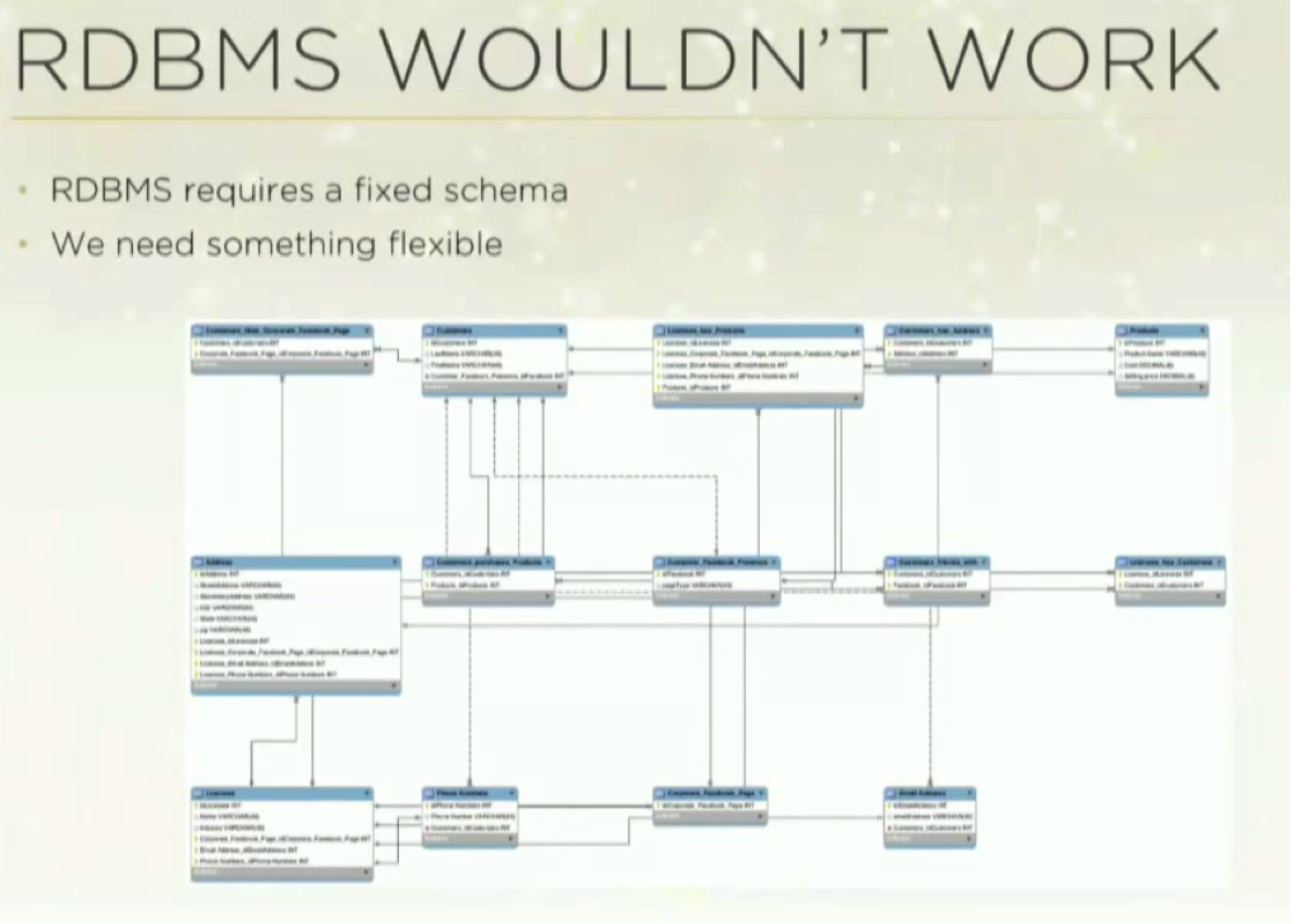
But we needed something more flexible than a relational model.
XML database
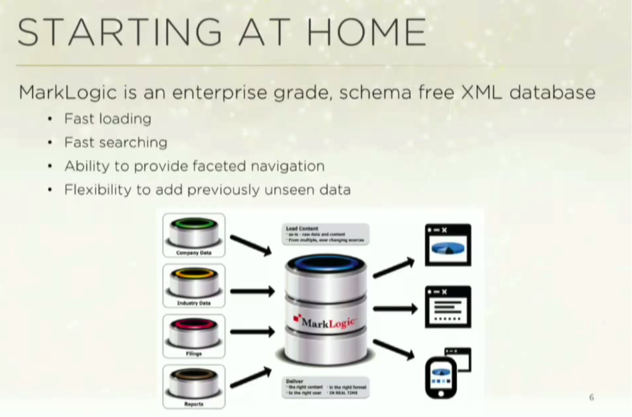
My prior experience was with NoSQL databases. At the time, I worked for a company called MarkLogic, an enterprise-grade schema-free XML database that also stores documents and does JSON. The database was fast, both in terms of uploading information and performing searches, and it was also schema-free:
While we did learn from this initial point of concept (POC), POCs are, by definition, a limited vision. We tested one subset of the grand vision at a time, took some sample sets and were able to do fast searches and navigations.
What we realized was that the implicit information between the documents was much more interesting that the information stored within each document. So we tried to figure out if we could build a database that allowed us to explore these relationships.
Again, we were modeling our information as documents, which suited our dataset well. But when you’re working with a document database, what you really care about is — of course — the documents. So while we could do JOINS, it just didn’t work for large datasets.
We could do fast searches within documents, but not the relationships between them. It just wasn’t the right tool for the job.
Resource Description Framework (RDF) / triple stores
As a solution, MarkLogic migrated all of our documents from XML to Resource Description Framework (RDF), also known as a triple store. While this was a big move and a very different way of looking at data, we determined it was the right thing to do.
It wasn’t too difficult a task because we very deliberately decoupled our persistence layer from the rest of the architecture. It took about two months, and we were able to perform the migration without really impacting the rest of the application.
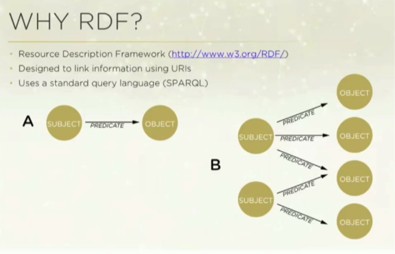
Why did we choose RDF? Because it’s designed to link information with uniform resource identifiers (URI), and it has a standard query language called SPARQL.
Very briefly, RDF is about subject/predicate/object relationships which you can see modeled very simply below:
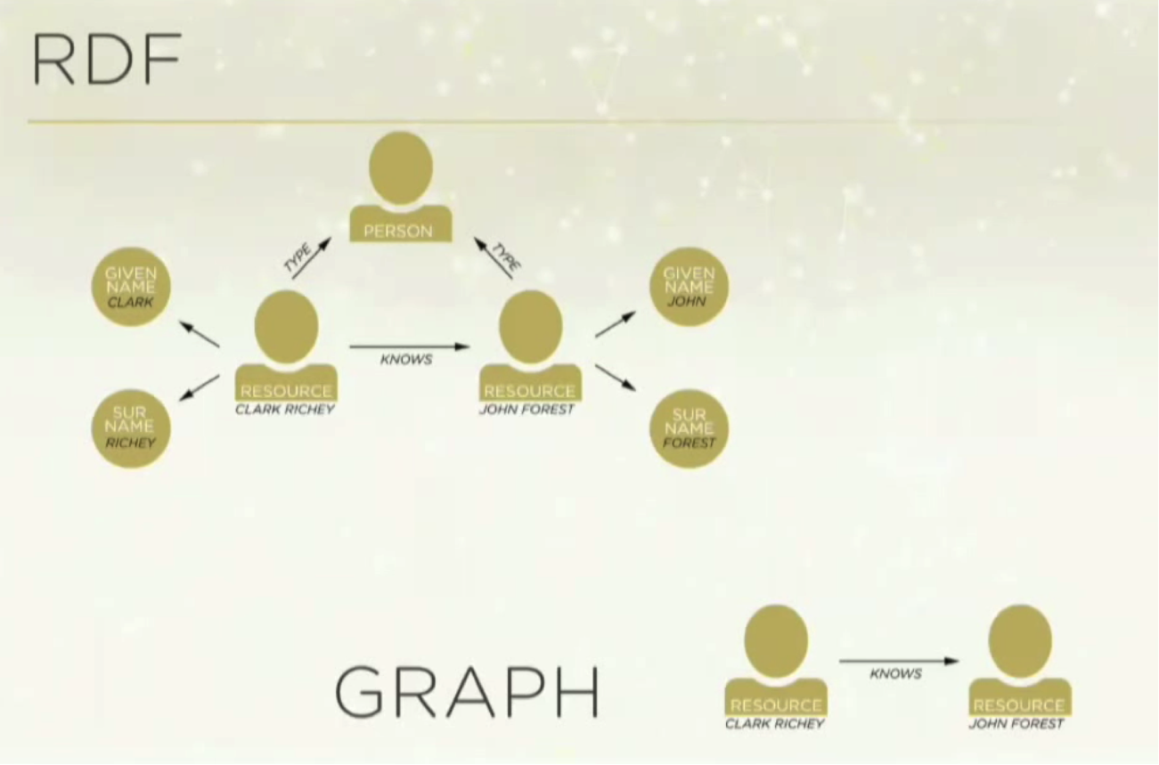
Below is a basic pictograph of the RDF concept:
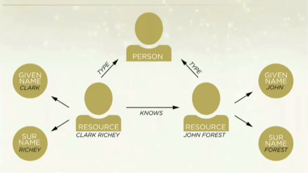
If I want to say Clark knows John Forrest, Clark is called the resource. The resource has properties such as a given name, a surname and a type, and also has relationships. Below are some RDF triples that represent this pictorial example:

We had a really powerful database, and were overall pretty pleased with it. We rebuilt our whole POC using RDF, and it allowed us to do a lot more with our database — including exploring relationships. And while it was very good for sharing data on a large scale amongst different organizations and industries, that wasn’t the main purpose of our database.
RDF is very verbose; it’s a non-properties based graph. And because everything is a node, complex queries of relationships required you to walk and join on a walk back which caused us some performance issues. And while RDF ultimately wasn’t the right tool for us, it did help us see the possibilities inherent in focusing on data relationships.
As a small startup, we were concerned that we had gone through so many databases in such a short time. Even so, we knew how important it was the choose the right database from the very beginning, so despite the pressure to try and make our insufficient database work, we decided to explore graph databases.
Making the switch: graph databases
At first, we thought graph databases were going to be just like RDF. But we knew that to describe a relationship between two people, RDF was too complicated. We wanted something much more simplistic that allowed us to assign properties to nodes, and we found this in a property graph model:
Again, we knew we couldn’t use a relational database because they don’t do relationships well. JOINS, foreign keys and indexes aren’t real or concrete; they’re just pictures we put on paper to understand them better. Conversely, in graph databases, relationships are conveyed as concrete entities.
TitanDB
We first explored TitanDB, which was very exciting at first because it had a powerful set of features with extreme scalability. Unfortunately it was very complex to launch and maintain because you had to run it off of either a Cassandra or HBase backend.
The other concerning feature were the eventual consistent stores, which were not ACID compliant. This meant that if we were to run a large graph database for a long period of time, it would become inconsistent.
TitanDB did provide a tool that was essentially a long-running process that consistently walked the entire graph to detect and fix inconsistencies. In addition to these inconsistencies, the program also applied it as a layer on top of a native store that wasn’t graph based.
OrientDB
Next we checked out OrientDB, which seemed much easier to launch and had a lot of document-centric features. But based on reviews in the community, performance and scalability seemed to be an issue. Additionally, they were marketing themselves as a multi-model database — graph and SQL. This lack of focus on pure graph operations concerned me; we wanted to do graphs, and do graphs well.
Finding Neo4j
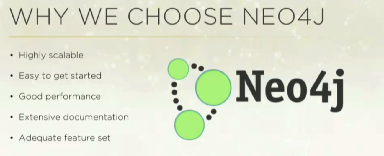
And then we found Neo4j. It was highly scalable with no limit on the number of nodes, relationships or indexes. It was also very easy to get started, which was a huge deal for us; when you’re working on your third database, you have to get up and running very quickly.
Performance was excellent, the augmentation was extensive, and it was focused solely on the graph use case. While Titan did offer support for maps as a native node type, we knew we could get by without that.
In summary, below are the reasons we chose Neo4j:
We’ve been on the Enterprise Edition of Neo4j for about 16 months, and our experience has been fantastic. It’s easy to use, easy to set up and maintain, and it delivered or exceeded all of our expectations. It enabled us to get beyond our POC, get into production and to build new things very, very quickly.
What we learned after the transition to Neo4j
Below are a number of helpful tips for running Neo4j:
1. If You’re a Java Shop, Run Neo4j Embedded
Since Neo4j is a native Java platform, and we are a Java shop, Neo4j was great for us. Embedding Neo4j allowed us to stop making REST calls, which is really important for security reasons. For more on the dangers of making REST calls, you can watch this JavaOne talk on REST security vulnerabilities.
Running Neo4j embedded also significantly reduced complexity for us. You can directly call out to the Neo4j API in process, which allowed us to quickly get started on Cypher, and it allowed us to run a combination of Cypher and the Java API. It also eliminated our need for both managed and unmanaged extensions.
2. Understand your strengths
It’s extremely important to understand your strengths as well as those of the tool you choose. If you try to use a tool for the wrong thing, it won’t perform well.
Native graph databases are really good with relationships; you find a starting point in the graph and explore relationships as deeply as you want, which is blazing fast with Neo4j. But if you want to do a complex, full-text and multi-value property searches off a single node, it won’t perform well — but then again, that’s not why you chose a graph database.
3. Understand what happens when you query
It is extremely important to know what happens when you query so that you can optimize your Cypher.
Below is a very simplified query to consider. I want to find each male in Franklin County who has a hunting license, and the address on the license needs to match the person’s home address so we know it’s the same person.
I have a person node, a license node and a place node, and there are different properties on each node:
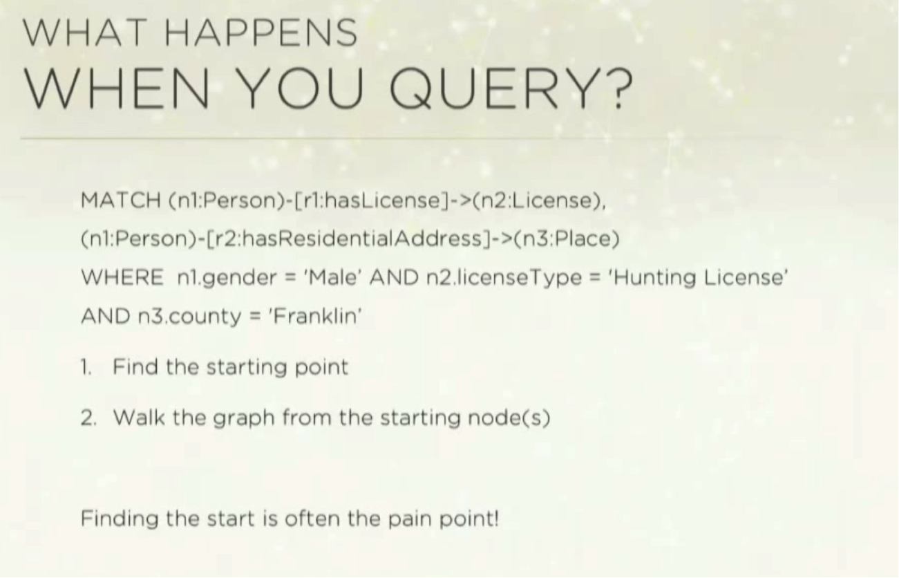
The first thing the database will do is find a starting point – for which there can be multiple – out from which the graph searches. Finding this starting point is very often the pain point. To remedy this, there is a rule-based planner with a static set of indexes that has more recently been upgraded to a
Indexes
Indexes are essentially duplicate pieces of information in the database that help it rapidly find nodes. In this case, it’s only used for identifying the starting point. While using indexes isn’t required, it’s very helpful. If you’re going to be searching on a certain node property, it’s a good idea to set an index on it, even though it will take up room on your disk.
There are two types of indexes: schema and legacy. Schema indexes are the newest and use internal custom Neo4j indexing built in house, and they are currently the default.
Once you create schema indexes via Cypher or the Java API, they’re automatically maintained by the database. For example, if you want to create an index on every node with the label “person” and the property “gender,” when you create a new node, change the value of the node or delete a node, the database will automatically update them. You can also now have constraints, such as a property must exist or be unique.
Legacy indexes are Lucene indexes, which are older but not deprecated. They can be configured via a configuration file, a Neo4j properties file, the Java API or Cypher. The legacy indexes use Lucene instead of the proprietary Neo4j indexing mechanism. While we have had very few bugs with Neo4j, almost every time we’ve come across one it has been related to the legacy index. Even so, sometimes these indexes are necessary.
Apache Luke is a great open source tool that allows you to directly view and search Lucene indexes. This has helped us fix odd behavior in our legacy indexes.
Automatic versus Manual Indexing
There are two ways to use legacy indexes: auto indexing and manual indexing. I would recommend using auto indexing because it’s easier to maintain. You essentially set it up once — either in the configuration file or through the API — and set it to index a certain type of property on a certain type of node. It also allows you to easily rebuild indexes if necessary.
However, you aren’t able to specify what type of index it is. In Lucene, the schema have different index types — such as string, case sensitive and numeric — which are actually physically separate indexes.
When you query Lucene and you want to use those indexes, the first thing you have to do is tell Lucene which index to use. But when you do auto indexing, Neo4j can choose which index to use based on the first thing you index. For example, if the first index you set is blue, and Neo4j knows that blue is a string, it will permanently place it in the string index.
This works well if you have good control over the data coming in. However, our system does not. We accept data from a huge variety of sources, so that “blue” property that came in may refer to an age. But if that’s the first thing that came in, Neo4j is going to index age as a string-based property rather than a numeric property, which will prevent my future comparisons and ranges from working in the way that I want. In this case, you will have to manually create the indexes.
Another benefit to using auto indexing is that it’s easy to fix the directory if it somehow becomes corrupted. You can stop the whole database, go into the Lucene index directory, delete it, restart the database and Neo4j will re-index all the nodes. But if you’ve done manual indexing, you’ll have to go back and re-index all the nodes.
Range Queries
Below is a series of slides that show range queries:

Because I want to query “profile”, I put PROFILE at the front of the query. I want to find all the people who have an income of a certain value — 50,500 — and only return the first two results.
The code shows that I have an index on a person’s income, and the planner has a limit of two. NodeIndexSeek is using the index to look up that value, and it hits roughly 2800 database accesses out of a sample database of 220,000 people.
In the next range query, I’m looking for people who make less than 50,500:
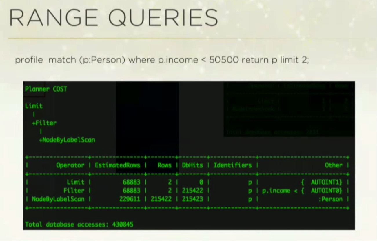
In this one, we do a NodeByLabelScan, and we get up to 430,000 database hits because it doesn’t use the index. Prior to Neo4j version 2.3, the schema indexes didn’t support ranges, so you had to use a legacy index and directly query the Lucene index for it to work.
This has been fixed in version 2.3; now you do get a NodeIndexSeekByRange, which provides range indexes on schema labels:

4. Don’t Use the Internal Node ID
It is very tempting to use current node IDs, but this is a very bad idea because at some point, you will end up deleting things from your database. You can read more about the topic here.
Neo4j uses a log of increments. If you delete a node, eventually they flip over the node IDs so you can reuse the numbers. We use a combination of the node label plus a randomized UUID which provides an added layer of security if you expose your API eternally.
5. Data modeling is important
Your data model is at least as important as your queries. The following tutorials are very helpful:
Some relationships can be modeled by multiple relationship types or a property on a relationship. Both approaches may seem equally reasonable, but their performance can vary significantly. Be sure to check out this resource on the topic from GraphAware.
It’s the difference between defining a relationship between person and place with different types…

…versus saying there are three different types of properties:
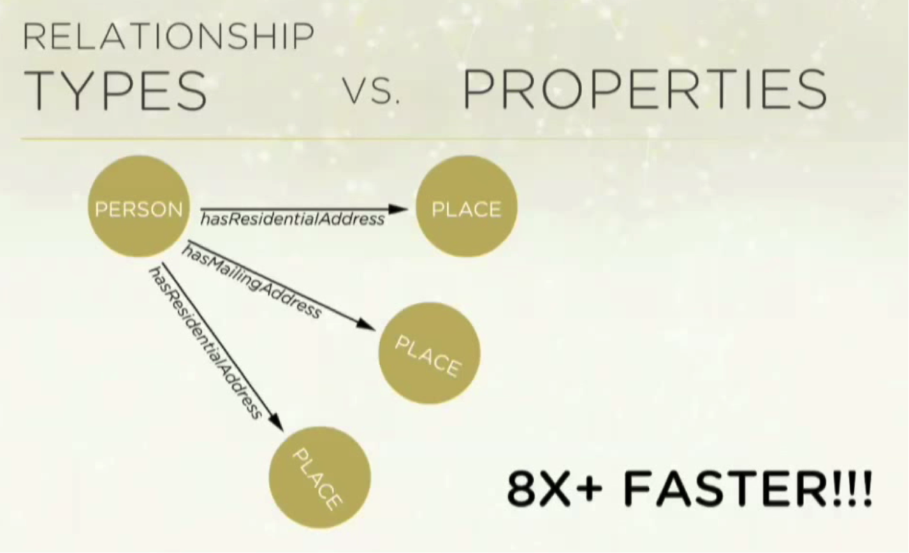
The performance increase can be by eight times faster. The GraphAware article referenced above explains this concept much more in depth.
6. Optimize performance
EXPLAIN and PROFILE are definitely your friends. Don’t be afraid of the Java API, but the query planner is still very young, and can be faster than Cypher in a lot of situations. When you’re benchmarking, it’s important to benchmark against a warm database. This allows Neo4j’s database caches to load.
7. Communicate!
Neo4j has great support community — it has Google groups, a Slack channel, Stack Overflow and an incredible support team.
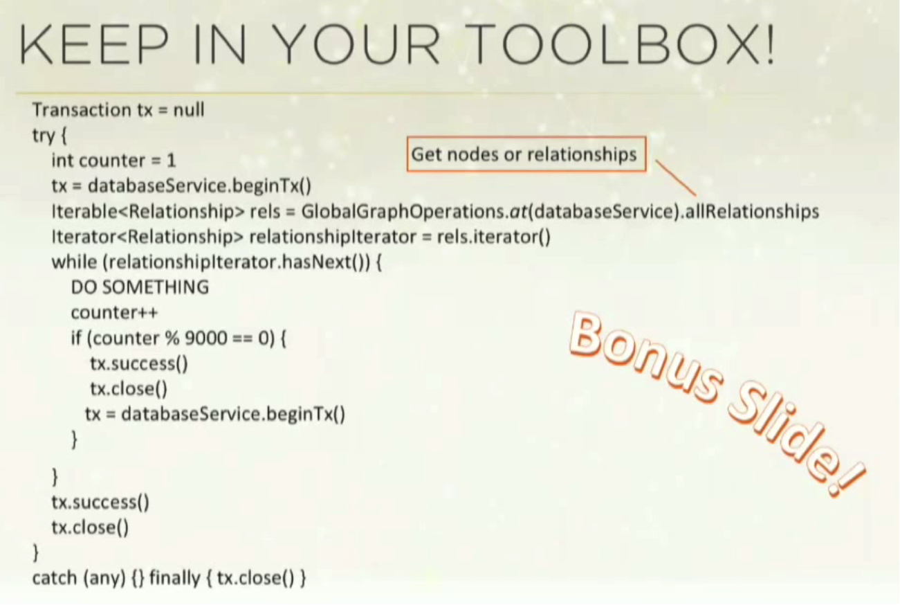
8. Keep this code in your toolbox
Below is some boilerplate code that allows you to go through each node in your database and fix any issues. This example happens to grab relationships, but you can do the same things for nodes or some other qualification.
Either way, it lets you loop through all the nodes in your database transactionally. In this case, it’s 90,000 operations per transaction, and it allows you to batch change the entire database if you need to:
Want to learn more about graph databases? Click below to get your free copy of O’Reilly’s Graph Databases ebook and start using graph technology in your next application.
Share Article


Explore
Related Articles

A workbench for teams to query, explore, and visualize graph data
Neo4j Named “One to Watch” in Snowflake’s 2026 Modern Marketing Data Stack Report
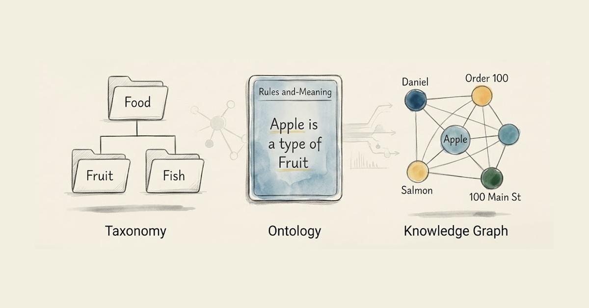
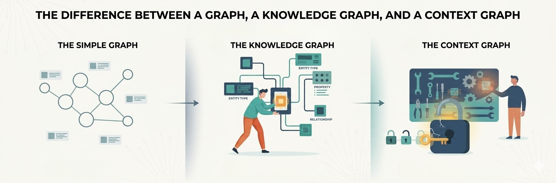
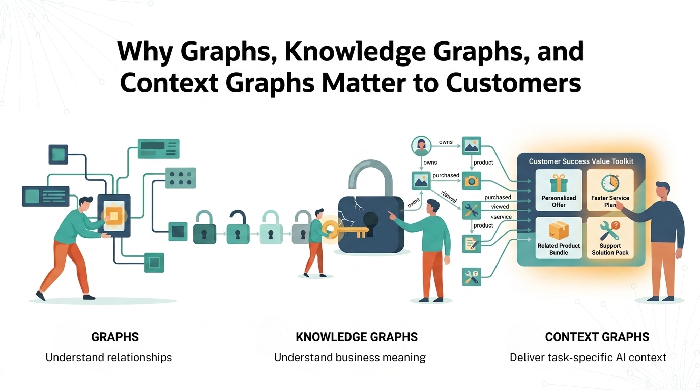
1 of 3: The difference between a graph, a knowledge graph, and a context graph