RDBMS & Graphs: Relational vs. Graph Data Modeling


12 min read
In some regards, graph databases are like the next generation of relational databases, but with first class support for “relationships,” or those implicit connections indicated via foreign keys in traditional relational databases.
Each node (entity or attribute) in a native graph property model directly and physically contains a list of relationship records that represent its relationships to other nodes. These relationship records are organized by type and direction and may hold additional attributes.
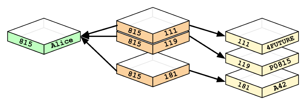
A graph/JOIN table hybrid showing the foreign key data relationships between the Persons and Departments tables in a relational database.
Whenever you run the equivalent of a JOIN operation, the database just uses this list and has direct access to the connected nodes, eliminating the need for a expensive search-and-match computation.
This ability to pre-materialize relationships into database structures allows graph databases like Neo4j to provide a minutes-to-milliseconds performance advantage of several orders of magnitude, especially for JOIN-heavy queries.
The resulting data models are much simpler and at the same time more expressive than those produced using traditional relational or other NoSQL databases.
In this RDBMS & Graphs blog series, we’ll explore how relational databases compare to their graph counterparts, including data models, query languages, deployment paradigms and more. In previous weeks, we explored why RDBMS aren’t always enough and graph basics for the relational developer.
This week, we’ll compare data modeling for both relational and graph data models.
Key Data Modeling Differences for RDBMS and Graphs
Graph databases support a very flexible and fine-grained data model that allows you to model and manage rich domains in an easy and intuitive way.
You more or less keep the data as it is in the real world: small, normalized, yet richly connected entities. This allows you to query and view your data from any imaginable point of interest, supporting many different use cases.
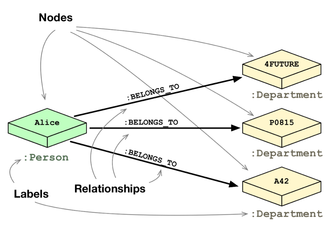
A graph data model of our original Persons and Departments data. Labeled nodes and relationships have replaced our tables, foreign keys and JOIN table.
The fine-grained model also means that there is no fixed boundary around aggregates, so the scope of update operations is provided by the application during the read or write operation. Transactions group a set of node and relationship updates into an Atomic, Consistent, Isolated and Durable (ACID) operation.
Graph databases like Neo4j fully support these transactional concepts, including write-ahead logs and recovery after abnormal termination, so you never lose your data that has been committed to the database.
If you’re experienced in modeling with relational databases, think of the ease and beauty of a well-done, normalized entity-relationship diagram: a simple, easy to understand model you can quickly whiteboard with your colleagues and domain experts. A graph is exactly that: a clear model of the domain, focused on the use cases you want to efficiently support.
Let’s take a model of the organizational domain and show how it would be modeled in a relational database vs. the graph database.
Brief Example: Organizational Data Domain
First up, our relational database model:
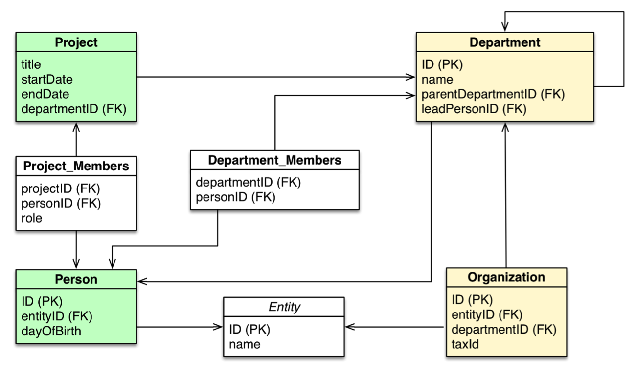
A relational database model of a domain with people and projects within an organization with several departments.
If we were to adapt this relational database model into a graph database model, we would go through the following checklist to help with the transformation:
- Each entity table is represented by a label on nodes
- Each row in a entity table is a node
- Columns on those tables become node properties
- Remove technical primary keys, but keep business primary keys
- Add unique constraints for business primary keys, and add indexes for frequent lookup attributes
- Replace foreign keys with relationships to the other table, remove them afterwards
- Remove data with default values, no need to store those
- Data in tables that is denormalized and duplicated might have to be pulled out into separate nodes to get a cleaner model
- Indexed column names might indicate an array property (like
email1,email2,email3) - JOIN tables are transformed into relationships, and columns on those tables become relationship properties
Once we’ve taken these steps to simplify our relational database model, here’s what the graph data model would look like:
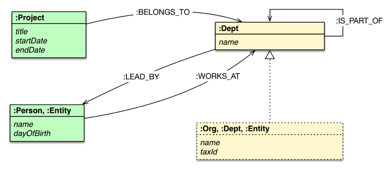
A graph data model of the same domain with people and projects within an organization with several departments. With the graph model, all of the initial JOIN tables have now become data relationships.
This above example is just one simplified comparison of a relational and graph data model. Now it’s time to dive deeper into a more extended example taken from a real-world use case.
In-Depth Example: Data Center Management
To show you the true power of graph data modeling, we’re going to look at how we model a domain using both relational- and graph-based techniques. You’re probably already familiar with RDBMS data modeling techniques, so this comparison will highlight a few similarities – and many differences.
In particular, we’ll uncover how easy it is to move from a conceptual graph model to a physical graph model, and how little the graph model distorts what we’re trying to represent versus the relational model.
To facilitate this comparison, we’ll examine a simple data center management domain. In this domain, several data centers support many applications on behalf of many customers using different pieces of infrastructure, from virtual machines to physical load balancers.
Here’s an example of a small data center domain:
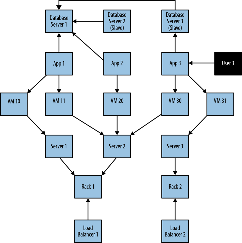
A simplified snapshot of several application deployments within a data center.
In this example above, we see a somewhat simplified view of several applications and the data center infrastructure necessary to support them. The applications, represented by nodes App 1, App 2 and App 3, depend on a cluster of databases labeled Database Server 1, 2, 3.
While users logically depend on the availability of an application and its data, there is additional physical infrastructure between the users and the application; this infrastructure includes virtual machines (Virtual Machine 10, 11, 20, 30, 31), real servers (Server 1, 2, 3), racks for the servers (Rack 1, 2) and load balancers (Load Balancer 1, 2), which front the apps.
Of course, between each of the components are many networking elements: cables, switches, patch panels, NICs (network interface controllers), power supplies, air conditioning and so on – all of which can fail at inconvenient times. To complete the picture we have a straw-man single user of Application 3, represented by User 3.
As the operators of such a data center domain, we have two primary concerns:
- Ongoing provision of functionality to meet (or exceed) a service-level agreement, including the ability to perform forward-looking analyses to determine single points of failure, and retrospective analyses to rapidly determine the cause of any customer complaints regarding the availability of service.
- Billing for resources consumed, including the cost of hardware, virtualization, network provisioning and even the costs of software development and operations (since these are simply logical extensions of the system we see here).
If we are building a data center management solution, we’ll want to ensure that the underlying data model allows us to store and query data in a way that efficiently addresses these primary concerns. We’ll also want to be able to update the underlying model as the application portfolio changes, the physical layout of the data center evolves and virtual machine instances migrate.
Given these needs and constraints, let’s see how the relational and graph models compare.
Creating the Relational Data Model
The first step in relational data modeling is the same as any other data modeling approach: to understand and agree on the entities in the domain, how they interrelate and the rules that govern their state transitions.
This initial stage is often informal, with plenty of whiteboard sketches and discussions between subject matter experts and data architects. These talks then usually result in diagrams like Figure 6 above (which also happens to be a graph).
The next step is to convert this initial whiteboard sketch into a more rigorous entity-relationship (E-R) diagram (which is another graph). Transforming the conceptual model into a logical model using a stricter notation gives us with a second chance to refine our domain vocabulary so that it can be shared with relational database specialists.
(It’s worth noting that adept RDBMS developers often skip directly to table design and normalization without using an intermediate E-R diagram.)
Here’s our sample E-R diagram below:
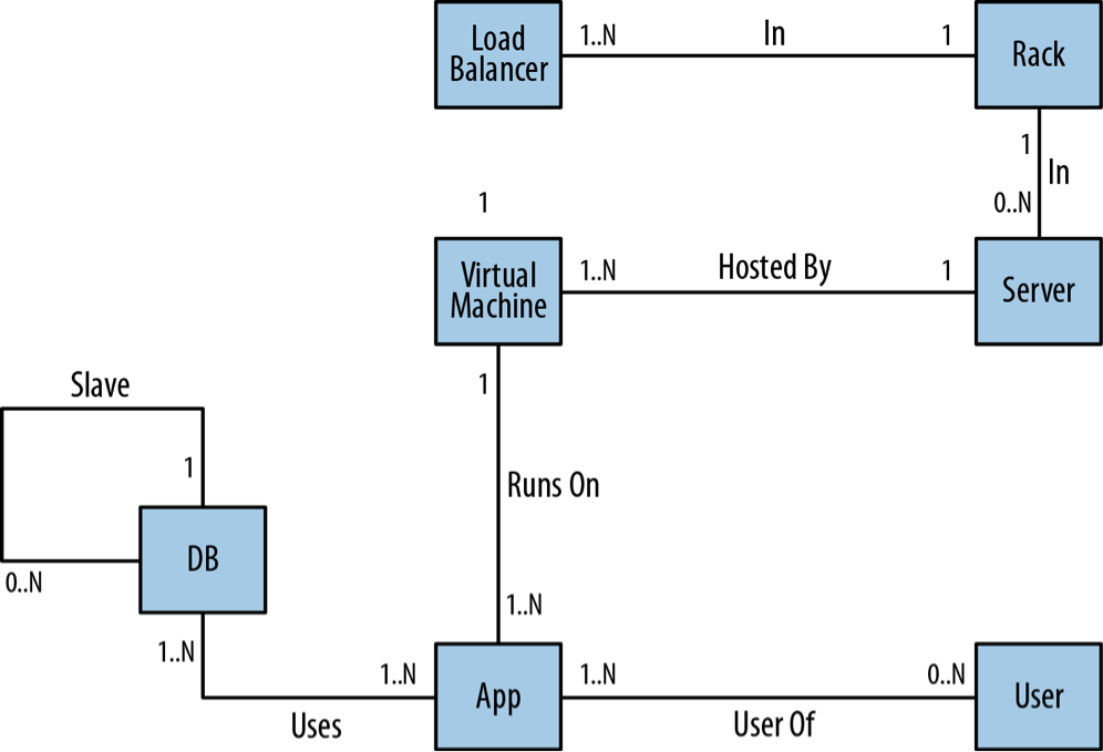
An entity-relationship (E-R) diagram for our data center domain.
Despite being graphs, E-R diagrams immediately show the shortcomings of the relational model. E-R diagrams allow only single, undirected relationships between entities. In this respect, the relational model is a poor fit for real-world domains where relationships between entities are both numerous and semantically rich.
Now with a logical model complete, it’s time to map it into tables and relations, which are normalized to eliminate data redundancy. In many cases, this step can be as simple as transcribing the E-R diagram into a tabular form and then loading those tables via SQL commands into the database.
But even the simplest case serves to highlight the idiosyncrasies of the relational model. For example, in the figure below we see that a great deal of accidental complexity has crept into the model in the form of foreign key constraints (everything annotated [FK]), which support one-to-many relationships, and JOIN tables (e.g., AppDatabase), which support many-to-many relationships – and all this before we’ve added a single row of real user data.

A full-fledged relational data model for our data center domain.
These constraints and complexities are model-level metadata that exist simply so that we specify the relations between tables at query time. Yet the presence of this structural data is keenly felt, because it clutters and obscures the domain data with data that serves the database, not the user.
The Problem of Relational Data Model Denormalization
So far, we now have a normalized relational data model that is relatively faithful to the domain, but our design work is not yet complete.
One of the challenges of the relational paradigm is that normalized models generally aren’t fast enough for real-world needs. In theory, a normalized schema is fit for answering any kind of ad hoc query we pose to the domain, but in practice, the model must be further adapted for specific access patterns.
In other words, to make relational databases perform well enough for regular application needs, we have to abandon any vestiges of true domain affinity and accept that we have to change the user’s data model to suit the database engine, not the user. This approach is called denormalization.
Denormalization involves duplicating data (substantially in some cases) in order to gain query performance.
For example, consider a batch of users and their contact details. A typical user often has several email addresses, which we would then usually store in a separate EMAIL table. However, to reduce the performance penalty of JOINing two tables, it’s quite common to add one or more columns within the USER table to store a user’s most important email addresses.
Assuming every developer on the project understands the denormalized data model and how it maps to their domain-centric code (which is a big assumption), denormalization is not a trivial task.
Often, development teams turn to an RDBMS expert to munge our normalized model into a denormalized one that aligns with the characteristics of the underlying RDBMS and physical storage tier. Doing all of this involves a substantial amount of data redundancy.
The Cost of Rapid Change in the Relational Model
It’s easy to think the design-normalize-denormalize process is acceptable because it’s only a one-off task. After the cost of this upfront work pays off across the lifetime of the system, right? Wrong.
While this one-off, upfront idea is appealing, it doesn’t match the reality of today’s agile development process. Systems change frequently – not only during development, but also during their production lifetimes.
Although the majority of systems spend most of their time in production environments, these environments are rarely stable. Business requirements change and regulatory requirements evolve, so our data models must too.
Adapting our relational database model then requires a structural change known as a migration. Migrations provide a structured, step-wise approach to database refactorings so it can evolve to meet changing requirements. Unlike code refactorings – which typically take a matter of minutes or seconds – database refactorings can take weeks or months to complete, with downtime for schema changes.
The bottom-line problem with the denormalized relational model is its resistance to the rapid evolution that today’s business demands from applications. As we’ve seen in this data center example, the changes imposed on the initial whiteboard model from start to finish create a widening gulf between the conceptual world and the way the data is physically laid out.
This conceptual-relational dissonance prevents business and other non-technical stakeholders from further collaborating on the evolution of the system. As a result, the evolution of the application lags significantly behind the evolution of the business.
Now that we’ve thoroughly examined the relational data modeling process, let’s turn to the graph data modeling approach.
Creating the Graph Data Model
As we’ve seen, relational data modeling divorces an application’s storage model from the conceptual worldview of its stakeholders.
Relational databases – with their rigid schemas and complex modeling characteristics – are not an especially good tool for supporting rapid change. What we need is a model that is closely aligned with the domain, but that doesn’t sacrifice performance, and that supports evolution while maintaining the integrity of the data as it undergoes rapid change and growth.
That model is the graph model. How, then, does the data modeling process differ? Let’s begin.
In the early stages of graph modeling, the work is similar to the relational approach: Using lo-fi methods like whiteboard sketches, we describe and agree upon the initial domain. After that, our data modeling methodologies diverge.
Once again, here is our example data center domain modeled on the whiteboard:
Our example data center domain with several application deployments.
Instead of turning our model into tables, our next step is to simply enrich our already graph-like structure. This enrichment aims to more accurately represent our application goals in the data model. In particular, we’ll capture relevant roles as labels, attributes as properties and connections to neighboring entities as relationships.
By enriching this first-round domain model with additional properties and relationships, we produce a graph model attuned to our data needs; that is, we build our model to answer the kinds of questions our application will ask of its data.
To polish off our developing graph data model, we just need to ensure correct semantic context. We do this by creating named and directed relationships between nodes to capture the structural aspects of our domain.
Logically, that’s all we need to do. No tables, no normalization, no denormalization. Once we have an accurate representation of our domain model, moving it into the database is trivial.
The Catch
So, what’s the catch? With a graph database, what you sketch on the whiteboard is typically what you store in the database. It’s that simple.
No catch.
After adding properties, labels and relationships, the resulting graph model for our data center scenario looks like this:
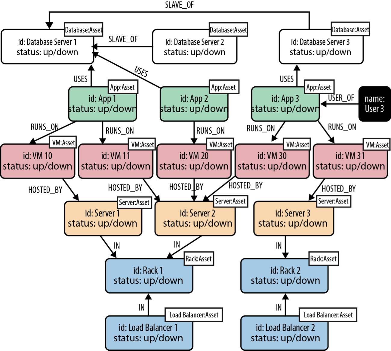
A full-fledged graph data model for our data center domain.
Note that most of the nodes here have two labels: both a specific type label (such as Database, App or Server), and a more general purpose Asset label. This allows us to target particular types of assets with some of our queries, and all assets – irrespective of type – with other queries.
Compared to the finished relational database model (included below), imagine which data model is easier to evolve, contains richer relationships and yet is still simple enough for business stakeholders to understand. We thought so.
A full-fledged relational data model for our data center domain. This data model is significantly more complex – and less user friendly – than our graph model on the preceding page.
Conclusion
Don’t forget: Data models are always changing. While it might be easy to dismiss an upfront modeling headache with the idea that you won’t ever have to do it again, today’s agile development practices will have you back at the whiteboard (or calling a migration expert) sooner than you think.
Even so, data modeling is only a part of the database development lifecycle. Being able to query your data easily and efficiently – which often means real-time – is just as important as having a rich and flexible data model.
Next week, we’ll examine the differences between RDBMS and graph database query languages.
Want to learn more on how relational databases compare to their graph counterparts? Download this ebook, The Definitive Guide to Graph Databases for the RDBMS Developer, and discover when and how to use graphs in conjunction with your relational database.
Catch up with the rest of the RDBMS & Graphs series:
- Why Relational Databases Aren’t Always Enough
- Graph Basics for the Relational Developer
- SQL vs. Cypher Query Languages
- 3 Database Deployment Strategies (Polyglot & More)
- Drivers for Connecting to a Graph Database
Share Article


Explore
Related Articles
From Data to Intelligence: Why Every Enterprise Needs an AI Knowledge Layer


Why Healthcare CIOs Can’t Afford to Scale AI Without a Knowledge Graph Foundation
Hey LLM, you’re using OPTIONAL MATCH wrong. Here’s the Cypher that actually works.