Getting from Denmark Hill to Gatwick Airport with Quantified Path Patterns

Software Engineer, Neo4j
16 min read

In this article, we are going to show how journey planning can be done using a dataset of the railway network in Great Britain and a new Cypher feature called quantified path patterns
Introduction
Planning a journey on a railway network is usually a simple matter of bringing up an app on a smartphone or visiting a website. These journey planners will probably use algorithms based on, for example, Scalable Transfer Patterns or A*.
It is very unlikely any of them use a brute force approach consisting of exhaustively finding all possible paths between A and B and ranking them according to some criteria like journey time; on a real-world dataset, this would never return in an acceptable amount of time.
But perhaps the brute force approach could be made to work if most paths could be eliminated up front based on some criteria.

We will be using a dataset of the railway network in Great Britain and apply a new Cypher feature called quantified path patterns (QPP). QPPs were introduced in Neo4j version 5.9, and perform the same function as the existing variable-length relationships, but it has a number of advantages:
- A more concise syntax.
- The repeating pattern to match can be made up of any number of nodes and relationships.
- Filters can be inlined, allowing unwanted results to be pruned as the graph is traversed.
It’s this last advantage that will enable us to return results fast enough for real-time journey planning.
Railway model
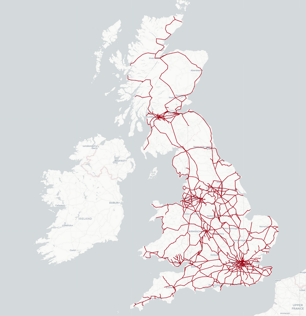
The data we’ll be using is extracted from publicly available datasets of the railway network in Great Britain. For those of you who want to try the queries, the extracted data is available here.
Here is what the data looks like on a map:
Here is a picture of the data model:
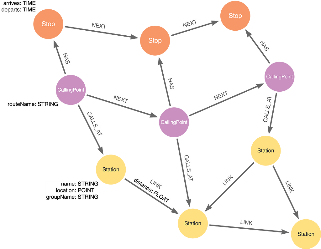
The model has three kinds of nodes:
- Station: The places where passengers begin and end their journeys, or change trains. They have a location property with the geographical coordinates of the station. Stations are connected to each other with LINK relationships, which have a property distance with the number of miles between the Stations.
- CallingPoint: Trains on the network follow a route, which is a sequence of Stations the trains call at. Each route is represented by a sequence of CallingPoints with a CALLS_AT relationship to the Stations.
- Stop: A timetable is made up of trains following a route at particular times. The arrival of a train is represented by a Stop with properties arriving and departs.
What do quantified path patterns look like?
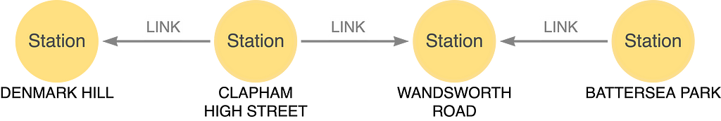
Let’s look at a simple example of a QPP. We start with a MATCH clause that finds all Station nodes that can be reached via a LINK from the Station called Denmark Hill:
MATCH (:Station {name: 'Denmark Hill'})-[link:LINK]-(:Station)
If we want to find all stations that are between one and four hops away from Denmark Hill, we can write the following QPP:
MATCH (:Station {name: 'Denmark Hill'}) (()-[l:LINK]-(s:Station)){1,4}
The pattern starts with an anchor node that matches the Station Denmark Hill. Following that is a QPP that matches the pattern ()-[:LINK]-(:Station) repeatedly. Each repetition follows a LINK relationship that ends on a Station node. The next repetition carries on from where the last one left off. Here is an example path that this would match:
This last fact is a key point and explains why putting the anchor node inside the QPP won’t work. For example, unless all Station nodes have the name “Denmark Hill,” the following will match at most a single hop:
MATCH ((:Station {name: 'Denmark Hill'})-[l:LINK]-(s:Station)){1,4}
For more details on the syntax, semantics, and path-matching machinery of QPPs, check out the Cypher documentation.
Minimal miles
Our first example will find the shortest distance between two Stations, Denmark Hill and Gatwick Airport (it’s a train station as well as an airport). Finding the shortest distance is not a simple case of finding a path with the fewest LINK relationships, as the distance between stations varies.
Our first stab at a brute-force solution does the following:
- Finds all paths between Denmark Hill and Gatwick Airport.
- Sums up the distance property of the LINK relationships.
- Sorts by total distance.
- Returns the first result.
The path will be composed of the following pattern repeated:
()-[:LINK]-()
We know our path will be made up of one or more of these patterns, so we wrap the above in parentheses with a + (which represents one or more repetitions):
(()-[:LINK]-())+
We also anchor the path at its ends with the start and finish stations:
(:Station {name: 'Denmark Hill'}) (()-[:LINK]-())+
  (:Station {name: 'Gatwick Airport'})
In order to compute the total distance, we need to add up the distance property of each LINK between the stations. To do this, we add the variable link to the QPP and then iterate over the list of LINK relationships in a reduce function:
MATCH (:Station {name: 'Denmark Hill'}) (()-[link:LINK]-())+
        (:Station {name: 'Gatwick Airport'})
RETURN reduce(acc = 0.0, l IN link | round(acc + l.distance, 2)) AS total
Finally, we sort by the totalDistance and return the top answer, as well as produce a list of the Station nodes so we know what the best route is:
MATCH p = (:Station {name: 'Denmark Hill'}) (()-[link:LINK]-())+
            (:Station {name: 'Gatwick Airport'})
RETURN reduce(acc = 0.0, l IN link | round(acc + l.distance, 2)) AS total,
  [n in nodes(p) | n.name] AS stations
ORDER BY total
LIMIT 1
With no upper bound to the path length, however, it should be no surprise that this query does not perform well — if it returns at all before running out of memory. As the data represents a real-world graph, the number of paths between two stations grows exponentially with the number of relationships.
We can check this is the case by running the following:
MATCH p = (:Station {name: 'Denmark Hill'}) (()-[link:LINK]-()){1,28}
            (:Station {name: 'Gatwick Airport'})
RETURN size(relationships(p)) AS numStations, count(*) AS numRoutes
ORDER BY numStations
We’ve added an upper limit of 28, as we only need to look at the trend, and want the query to return in a reasonable amount of time. Here are the results:
We can see a little bit more about what is happening by looking at one of the routes matched by our query:
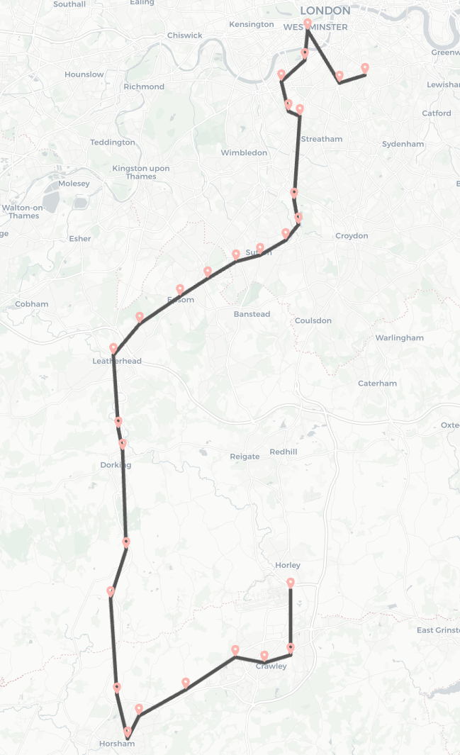
This is clearly not an optimal solution as it spends a fair amount of time not progressing towards its destination. The railway network in the south of the UK is fairly dense, so it should be possible to find a route that always moves in the right direction, allowing for some minimal diversions along the way.
With this insight, let’s add a filter that stops any traversal that moves too far in the wrong direction. We first need to add variables to the left-hand l and right-hand r nodes inside the QPP:
((l)-[link:LINK]-(r))+
We need a reference to the destination, Gatwick Airport, which we’ll use the variable gtw for. With these three variables, we can then write a filter using the spatial function point.distance to check if we are getting closer to Gatwick, give or take 1000 meters:
point.distance(r.location, gtw.location)
  - point.distance(l.location, gtw.location) < 1000
The variable gtw needs to be bound in a previous MATCH clause.
Putting it all together, we get:
MATCH (gtw:Station {name: 'Gatwick Airport'})
MATCH p = (:Station {name: 'Denmark Hill'})
          ((l)-[link:LINK]-(r) WHERE point.distance(r.location, gtw.location)
             - point.distance(l.location, gtw.location) < 1000)+ (gtw)
RETURN reduce(acc = 0.0, l IN link | round(acc + l.distance, 2)) AS total,
 [n in nodes(p) | n.name] AS stations
ORDER BY total
LIMIT 1
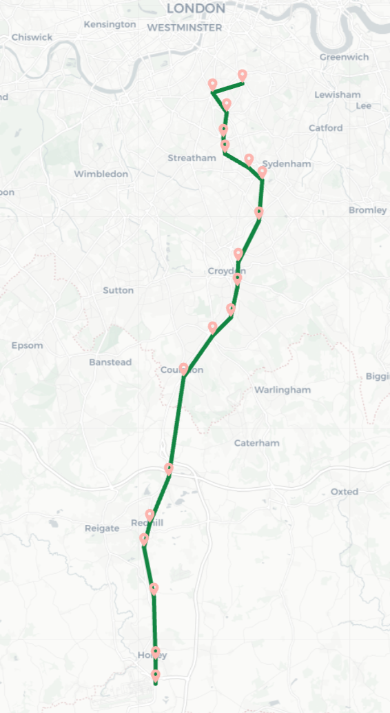
That’s better: we get a result, and we get it quickly (~20 ms when I run it on my laptop). Here it is on a map:
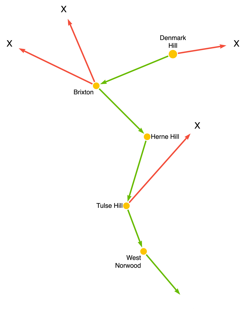
By placing a filter inside the QPP, we don’t waste time following relationships that we know can’t be part of our solution. The following picture visualizes this process, with the retained path in green, and the pruned traversals in red:
YMMV
Pruning variable-length traversals in Neo4j can also be done with variable-length relationships, but it’s less straightforward and is more restricted. Here is an example of a query with a variable-length relationship that can be pruned during traversal:
MATCH (a:Station)-[link:LINK*1..]->(b:Station)
WHERE all(l IN link WHERE endNode(l) <> a)
RETURN b.name
Because the function all() returns true if the condition holds for each iteration of the variable-length relationship, Cypher can apply the filter to each iteration.
But can we use this to replicate the QPP query above? No. In order to do that, we need to be able to compare the successive stations in order, from left to right. But the LINK relationships can point in any direction. This means the endNode() function (or its companion, the startNode() function) isn’t always going to give the right-hand node each time. By contrast, the pattern inside a QPP allows us to grab a reference to whichever node we need to unambiguously.
Mind the transfer
So far, the paths we’ve been finding assume a traveler can move along any stretch of track, much like a car on a road. But this is a railway, and the only way to get from A to B is to catch a train, and that train may or may not follow the desired route. The problem is then one of finding a train service whose route connects your start and finish stations, and then looking up the next arrival of a train on that route in a timetable. To do this, we now need to use another part of our data mode, the sequence of CallingPoint nodes, with the start and end nodes of those paths connecting to the start and finish Station nodes.
This is the shape our query needs to look for:
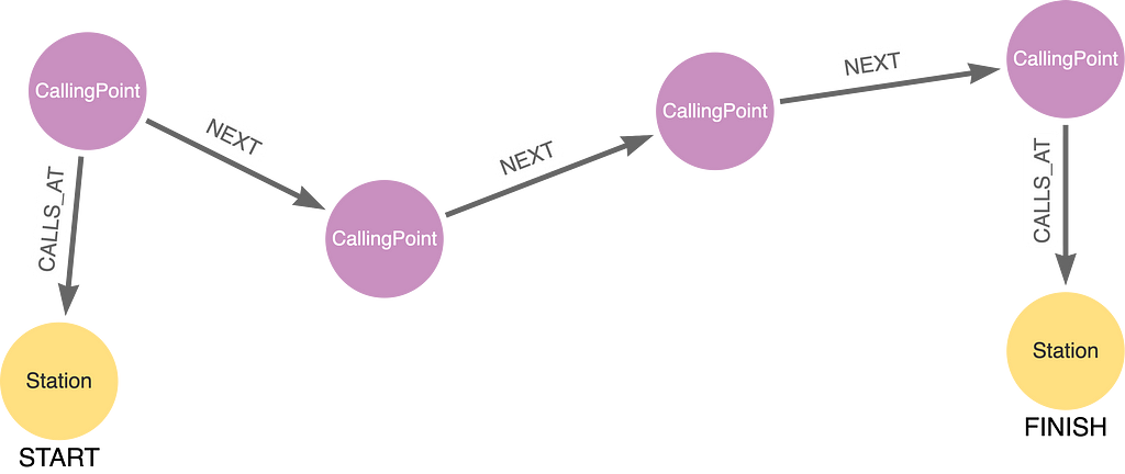
We piece together the above with a sequence of fixed-length path patterns and QPPs. We anchor the beginning with the CallingPoint at Denmark Hill:
(:Station {name: 'Denmark Hill'})<-[:CALLS_AT]-(r:CallingPoint)
And the end with the CallingPoint at Gatwick Airport:
(:CallingPoint)-[:CALLS_AT]->(:Station {name: 'Gatwick Airport'})
In the middle is a QPP that matches a variable length of CallingPoints connected by NEXT relationships:
(()-[:NEXT]->())+
Putting it together, we get:
MATCH (:Station {name: 'Denmark Hill'})<-[:CALLS_AT]-(r:CallingPoint)
        (()-[:NEXT]->())+
        (:CallingPoint)-[:CALLS_AT]->(:Station {name: 'Gatwick Airport'})
RETURN r.routeName AS route
If you run this query, however, you will get no results. It seems there are no direct trains from Denmark Hill to Gatwick Airport. Maybe we need to catch two trains. This is an example of two connecting train services:
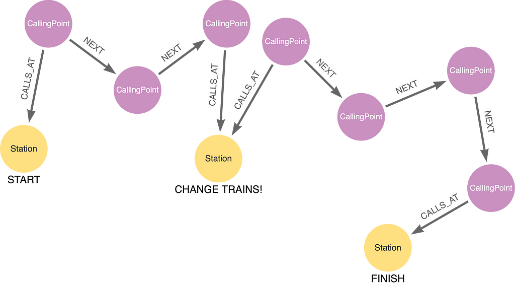
The changeover station is matched with a pattern that has CallingPoint nodes from two different services that call at the same Station node:
(:CallingPoint)-[:CALLS_AT]->(:Station)<-[:CALLS_AT]-(:CallingPoint)
Sandwiching this with patterns anchored at our start and destination Station nodes, we get:
MATCH (dmk:Station {name: 'Denmark Hill'})<-[:CALLS_AT]-(l1:CallingPoint)
  (()-[:NEXT]->())+
  (:CallingPoint)-[:CALLS_AT]->(x:Station)<-[:CALLS_AT]-(l2:CallingPoint)
  (()-[:NEXT]->())+
 (:CallingPoint)-[:CALLS_AT]->(gtw:Station {name: 'Gatwick Airport'})
RETURN l1.routeName AS leg1, x.name AS changeAt, l2.routeName AS leg2
This time, we get matches: 1248 pairs of routes that connect at 19 different stations. That’s a lot of routes to pick from, but we at least know we only need two trains to get from Denmark Hill to Gatwick Airport, and not three or more.
Now that we have candidate routes, we can check the timetable and select particular trains to catch. We need to give passengers enough time to make the connection, but also pick trains so they don’t have to wait at the changeover station for too long.
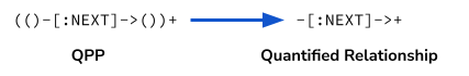
For concision, we’re going to introduce an abbreviated form of QPPs, called a quantified relationship. We can use this when we don’t need to declare any variables or predicates in the node patterns inside the QPP. In a quantified relationship, only the relationship pattern and quantifier remain:
The query starts with the MATCH clause above that returns our candidate routes, using compact quantified relationships:
MATCH (dmk:Station {name: 'Denmark Hill'})<-[:CALLS_AT]-(l1a:CallingPoint)-[:NEXT]->+
        (l1b)-[:CALLS_AT]->(x:Station)<-[:CALLS_AT]-(l2a:CallingPoint)-[:NEXT]->+
        (l2b)-[:CALLS_AT]->(gtw:Station {name: 'Gatwick Airport'})
We then connect those CallingPoint nodes to specific Stop nodes. You may recall from the beginning that Stop nodes represent the specific arrivals and departures of trains for a service. Here is the pattern for connecting a CallingPoint node to a Stop node (l1a is already bound in the first MATCH clause):
(l1a)-[:HAS]->(:Stop)
From this Stop node, we traverse across a variable number of NEXT relationships till we get to a Stop that is connected to the end CallingPoint, adding a filter on the departs time of the starting Stop:
(l1a)-[:HAS]->(s1:Stop)-[:NEXT]->+(s2)<-[:HAS]-(l1b)
  WHERE time('09:30') < s1.departs < time('10:00')
The pattern for the sequence of Stop nodes that make up the second leg of the journey are the same, but with a different filter that ensures passengers don’t wait more than 15 minutes when changing trains:
(l2a)-[:HAS]->(s3:Stop)-[:NEXT]->+(s4)<-[:HAS]-(l2b)
  WHERE s2.arrives < s3.departs < s2.arrives + duration('PT15M')
Assembling this into a single query that projects some useful information about the journey, we get:
MATCH (dmk:Station {name: 'Denmark Hill'})<-[:CALLS_AT]-(l1a:CallingPoint)-[:NEXT]->+
        (l1b)-[:CALLS_AT]->(x:Station)<-[:CALLS_AT]-(l2a:CallingPoint)-[:NEXT]->+
        (l2b)-[:CALLS_AT]->(gtw:Station {name: 'Gatwick Airport'})
MATCH (l1a)-[:HAS]->(s1:Stop)-[:NEXT]->+(s2)<-[:HAS]-(l1b)
        WHERE time('09:30') < s1.departs < time('10:00')
MATCH (l2a)-[:HAS]->(s3:Stop)-[:NEXT]->+(s4)<-[:HAS]-(l2b)
        WHERE s2.arrives < s3.departs < s2.arrives + duration('PT15M')
RETURN s1.departs AS leg1Departs, s2.arrives AS leg1Arrives, x.name AS changeAt,
         s3.departs AS leg2Departs, s4.arrives AS leg2Arrive,
         duration.between(s1.departs, s4.arrives).minutes AS journeyTime
ORDER BY leg2Arrive
LIMIT 5
The query returns five journeys, in ascending order of the arrival time at Gatwick Airport, taking about 100ms:
Not London calling
You can see from the changeAt column that several of the routes go via London terminals. Traveling via a London terminal costs more. To save money, we should filter out London terminal stations. To do this, we need to revert the quantified relationships to the full QPP form, so that we can add EXIST subqueries that filter out these routes:
MATCH (dmk:Station {name: 'Denmark Hill'})<-[:CALLS_AT]-(l1a:CallingPoint)
        (()-[:NEXT]->(n)
          WHERE NOT EXISTS { (n)-[:CALLS_AT]->(:Station:LondonGroup) })+
        (l1b)-[:CALLS_AT]->(x:Station)<-[:CALLS_AT]-(l2a:CallingPoint)
        (()-[:NEXT]->(m)
          WHERE NOT EXISTS { (m)-[:CALLS_AT]->(:Station:LondonGroup) })+
        (l2b)-[:CALLS_AT]->(gtw:Station {name: 'Gatwick Airport'})
MATCH (l1a)-[:HAS]->(s1:Stop)-[:NEXT]->+(s2)<-[:HAS]-(l1b)
WHERE time('09:30') < s1.departs < time('10:00')
MATCH (l2a)-[:HAS]->(s3:Stop)-[:NEXT]->+(s4)<-[:HAS]-(l2b)
WHERE s2.arrives < s3.departs < s2.arrives + duration('PT15M')
RETURN s1.departs AS leg1Departs, s2.arrives AS leg1Arrives, x.name AS changeAt,
        s3.departs AS leg2Departs, s4.arrives AS leg2Arrive,
        duration.between(s1.departs, s4.arrives).minutes AS journeyTime
ORDER BY leg2Arrive
LIMIT 5
Now, all the routes go via the same route:
Adding the additional filter to eliminate the London routes significantly improves the query performance, in fact, by 10–20 times faster. A nice illustration of the benefits of inlining filters into QPPs.
You have arrived
Hopefully, this article has convinced you of the usefulness of quantified path patterns. The examples showed how being able to inline filters lets you be more explicit about the kind of pruning you want Cypher to do and avoid wasteful traversals. And because any repeating pattern can be used, the filters you can write can be more specific, letting you compare neighboring nodes, call EXIST subqueries, and so on. Try it out in your own projects, or using the example railway dataset.
Getting from Denmark Hill to Gatwick Airport with quantified path patterns was originally published in Neo4j Developer Blog on Medium, where people are continuing the conversation by highlighting and responding to this story.
Share Article


Explore
Related Articles

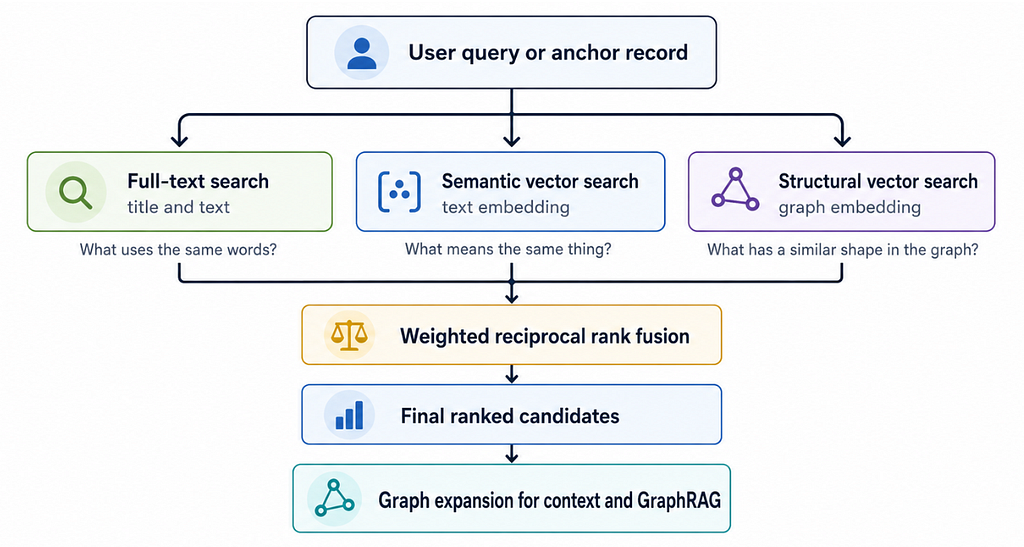
Hybrid Search in Neo4j: Full-Text, Vectors, and Graph Topology with Cypher