Exploring Fraud Detection With Neo4j & Graph Data Science – Part 4

Data Science Product Specialist, Neo4j
8 min read

In the three previous parts of this series, we explored the graph, identified new fraud risk accounts and communities, and covered techniques to recommend new suspicious users. In this section, we will cover how to apply graph machine learning to predict the high fraud risk user accounts we labeled in the previous parts of this series.
The technical resources to reproduce this analysis and the analysis in all other parts of this series are contained in this GitHub repository, which includes an iPython notebook and link to the dataset.
Motivation
In real-world scenarios we often don’t know which user accounts are fraudulent ahead of time. There will be cases, like with this dataset, where some accounts get flagged due to business rules — for example chargeback history, or via user reporting mechanisms. However, as we saw in parts 1 & 2 of this series, those flags don’t tell the whole story. The community detection and recommendation approaches we previously covered can go a very long way in helping us understand this story and label additional fraud risk users and patterns.
That said, there are multiple reasons why we may want to add supervised machine learning to predict the additional fraud risks:
- Proactive Detection: We can train a model to identify fraudulent actors ahead of time (such as before additional chargebacks or system flags) and better identify new communities that aren’t connected to older known fraud accounts.
- Measurable Performance: Supervised learning models produce clear performance metrics that enable us to evaluate and adjust as needed.
- Automation: Supervised machine learning automates the prediction of fraud risk accounts.
In the below sections, we will walk through how to engineer graph features for ML, export those features to Python, then train and evaluate an ML model for fraud classification.
Engineering Features for a Machine Learning Model
If we want a machine learning model to successfully classify fraud risk user accounts, we need to supply features that will be informative for the task. Below is a summary of the feature engineering strategy — you can find the full code in this notebook.
Building Features from Previous Analysis
From part 2 in this series we made communities out of shared Card relationships and shared Id relationships based on a provided set of business rules. Creating features out of those graph structures can be informative for machine learning. Below is a summary:
- Community Indicator and Size: Recall that flagged users tend to be in multi-user communities more often than non-flagged users. By definition, the new fraud risk users only exist in those communities. As such, it will likely be informative to add a (0,1) indicator feature for community size greater than one user, as well as a feature for total user count.
-
PageRank on P2P With Shared Card Degree: In part 1, we discovered the suspicious pattern of users sending money to accounts they share credit cards with. In part 2, we created the relationship
P2P_WITH_SHARED_CARDto mark this pattern between user pairs. It stands to reason that user accounts involved in P2P transactions with shared cards have a higher likelihood of being fraudulent. PageRank is a centrality algorithm that measures influence within a directed network.If we apply pageRank to the
P2P_WITH_SHARED_CARDrelationships and user nodes it could make a valuable feature for our machine learning model. - Degree Centrality on the Shared Id Rule: In part 2 we also created the
SHARED_IDSrelationships between users that share a strong pattern of shared credit cards, devices, and/or IP addresses. This data set has many instances of shared identifiers. Some of these instances may be benign (you can imagine some situations, such as sharing between family members, where this could be okay), but large frequencies are suspect and could be a sign of third-party fraud. The degree centrality of user nodeSHARED_IDSrelationships can therefore make a valuable feature for machine learning.
Other Useful Centrality Features
- P2P weighted Degree Centrality and PageRank: Out-degree and in-degree centrality on the P2P relationships weighted by the amount sent will translate to total P2P money sent and received respectively.
PageRank can be interpreted as a measure of how much money from all the P2P transactions “flows” through a given user node. These metrics can be informative if we expect fraud accounts to move more money than the average user. As such, we will include them as features for machine learning.
- Degree Centrality for Cards, Devices, and IPs: The total number of each identifier a user has may be indicative of fraud. In third-party fraud for example, a user may have many more cards and/or devices than normal connected to their account since they are using the identities of other people. We will include these centrality metrics as features for our our model.
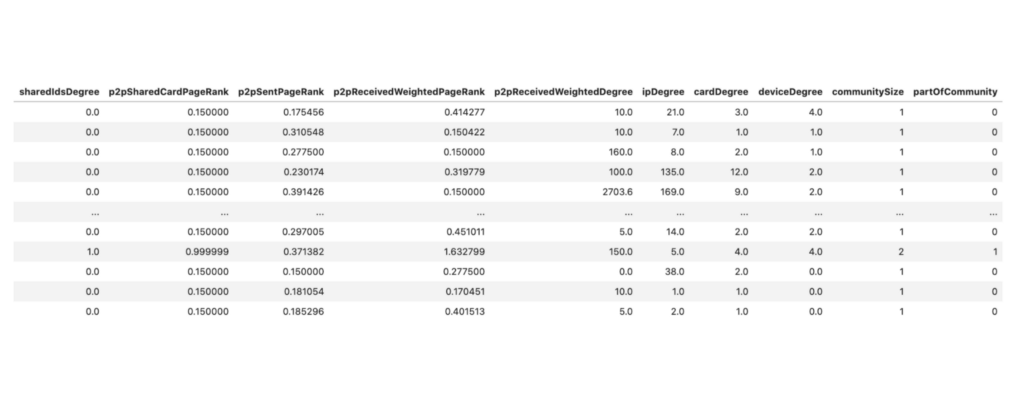
Once we calculate the features they will look something like this:
Machine Learning in Python
Below are commands to read the user data into Python and define the feature matrix, X, and the output class vector y. Note that my calculation for y means that the fraud class we are trying to predict is defined as just the newly identified fraud risks from part 2 — excluding the original flagged “fraudMoneyTransfer” users. We could easily write models to predict both types. However, designing a machine learning model for the newly labeled data exclusively could prove more valuable.
A model that predicts the original flagged user accounts will not be useful if it can only classify those accounts after they have done significant damage in the form of transacting a lot of money and incurring significant chargebacks on the platform — which is the situation we have here. There are some more complex temporal techniques we could explore for these — perhaps a subject for another blog. In general though, we are likely better off predicting the newly labeled fraud risks, at least to start.
These accounts are connected to the flagged chargeback accounts by definition, so successfully predicting them can help us more proactively identify fraudulent actors and communities before significant chargebacks have taken place. Recall also that these accounts went unnoticed/unflagged prior to examining in graph — as such, graph is specifically well-suited for identifying these cases.
df = gds.run_cypher('''
    MATCH(u:User)
    RETURN u.guid AS guid,
        u.wccId AS wccId,
        u.fraudRisk AS fraudRisk,
        u.fraudMoneyTransfer AS fraudMoneyTransfer,
        u.sharedIdsDegree AS sharedIdsDegree,
        u.p2pSharedCardPageRank AS p2pSharedCardPageRank,
        u.p2pSentPageRank AS p2pSentPageRank,
        u.p2pReceivedWeightedPageRank AS p2pReceivedWeightedPageRank,
        u.p2pReceivedWeightedDegree AS p2pReceivedWeightedDegree,
        u.ipDegree AS ipDegree,
        u.cardDegree AS cardDegree,
        u.deviceDegree AS deviceDegree,
        u.communitySize AS communitySize,
        u.partOfCommunity AS partOfCommunity
''')

X = df.drop(columns=['fraudRisk', 'fraudMoneyTransfer', 'wccId', 'guid'])

y = df.fraudRisk - df.fraudMoneyTransfer
For purposes of this demo I am going to use a random forest classifier. Other classifiers including logistic regression, SVM, Neural Nets, and Boosting variants could work as well. Going into the exact pros and cons of these models is out of scope here. Overall, I like exploring classification with random forests since they are relatively robust to feature scaling and collinearity issues and require minimal tuning to get working well.
Running the random forest with fairly minimal configuration yields promising results for a first pass. You can find the full code in the notebook. Below are some of the outputs.
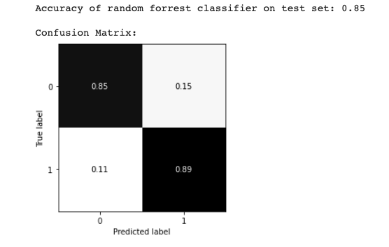
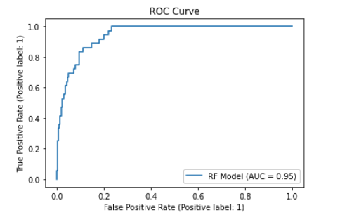
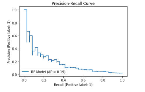
We can see total accuracy of around 85 percent. The AUCPR measures the trade-off between precision and recall. This is an important metric to look at for fraud classification use cases since the problem tends to be highly imbalanced (only a small set of fraudsters relative to other users). As such the AUCPR will generally be lower than AUC based on ROC and give you a better picture of the false-positive vs true-positive trade-off you would expect when applying the model in a production setting.
Of course this is just a quick demo example. The model could be improved with better labeling, more data, features, modeling tuning, etc.
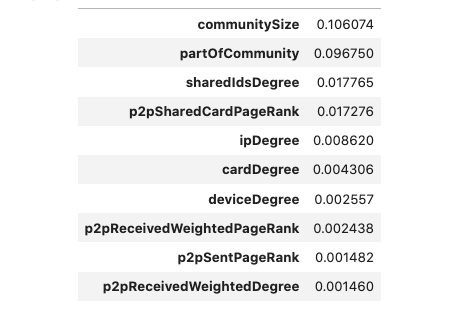
Below is a ranked list of the most influential features. Among the most important are the community sizes and the shared ids degree and p2p shared card pageRank.
Investigating Unlabeled High-Probability Fraud Risk Predictions
The labeling from part 2 wasn’t perfect.
Now that we have trained a machine learning model, investigating user accounts that were predicted as high probability fraud risks despite not being labeled as such by us (ostensible false positives), will bring further insights. Below are a couple examples from the test set visualized in Neo4j Bloom. The larger, leftmost, green nodes with user icons represent the high probability nodes of interest.
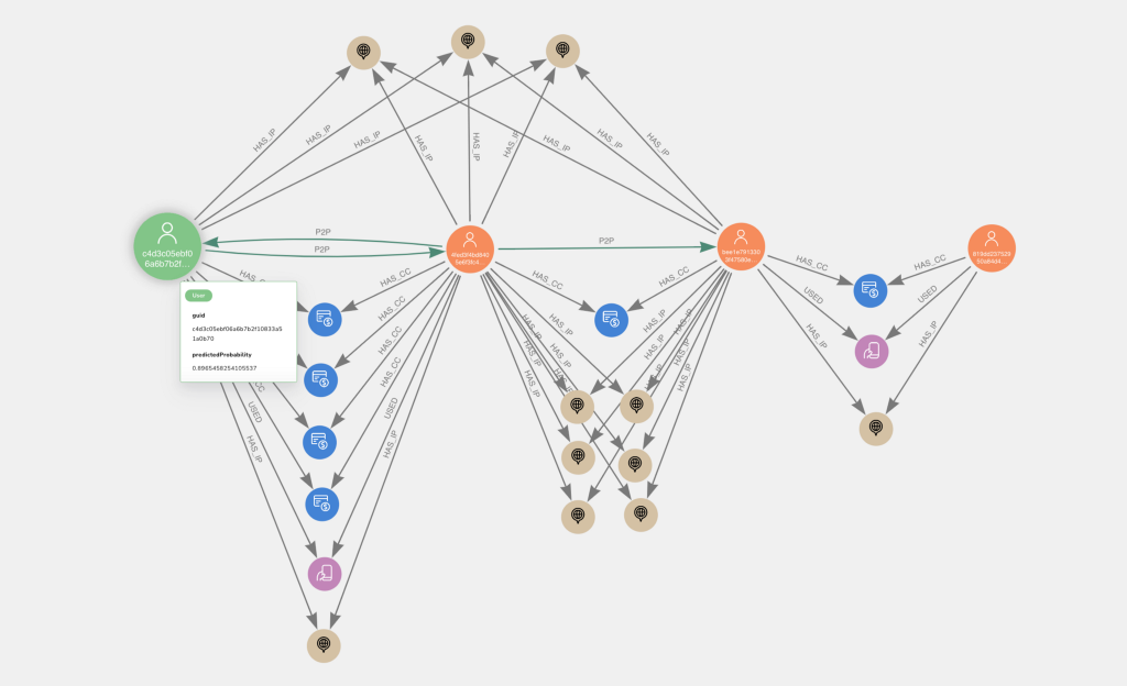
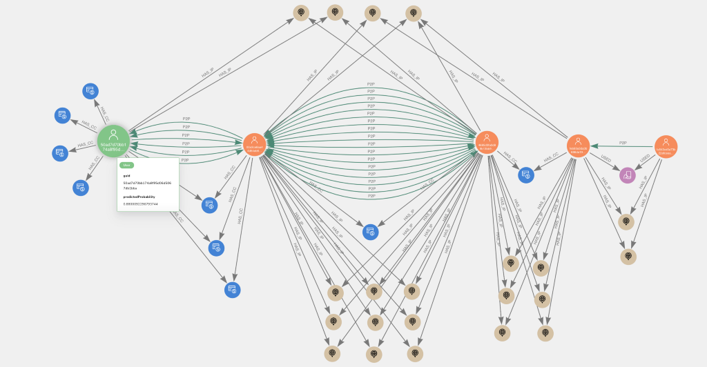
Perhaps unsurprisingly, they exhibit the P2P with shared card behavior. They also have a relatively large number of credit cards (the median degree centrality on cards is 3).
This could potentially be a sign of fraud, though it is hard to know on an anonymized dataset like this.
This is where subject matter expert review and iteration comes in. If this behavior turns out to be a clear indicator of fraud, it means we are predicting fraud more proactively before chargebacks take place, which is the ideal. In this case, if we re-label these users appropriately and re-train our ML model as more data comes in, we will further improve predictive performance. If, on the other hand, it turns out that some of this behavior is benign, we can adjust the feature engineer and model so the ML learns to rule out such cases which will likewise improve predictive performance and increase our understanding of fraud patterns. Either way, it is a win.
Conclusions
In this final part of the fraud detection series we demonstrated how easy it is to engineer graph features and create a supervised machine learning model to predict fraud risk user accounts. In doing so, we can investigate and hone our machine learning capabilities to proactively predict fraud and improve our understanding of fraud patterns.
This takes us to the end of our graph data science journey in this series. We explored the graph to find potential fraud patterns, used those findings to execute graph algorithms that resolved and labeled communities of fraud risk users, leveraged further graph analytics to recommend suspect user accounts that are similar to those in our resolved communities, then finally applied supervised machine learning to predict fraud risk accounts. While we focused on an anonymized sample of P2P data here, these methods are highly transferable to other fraud detection use cases.
Time provided in the future, I will cover some more of these. Until then, I hope this series has been of use for you.
As mentioned throughout this series there is a notebook that contains code for reproducing the analysis. That notebook and a link to the data which should allow you to reproduce the analysis in all four parts end-to-end are located in this GitHub repository.
A big thank you to Jaimie Chung for helping edit this series.
Here’s your key to the whole series:
Share Article


Explore
Related Articles


How to Improve Multi-Hop Reasoning With Knowledge Graphs and LLMs