Using a Graph Recommendation Algorithm for Predicting Chemical – Cell Interaction

Back End Developer at CytoSMART
8 min read
Recommendation algorithms are often written with a user-product relationship in mind. “Which user bought what product” or “Who liked this movie”. From this data, a prediction is made about an unknown user-product relation. However, this same algorithm can predict reactions between a chemical and a specific cell line.
In this blog, I will implement a Collaborative filtering algorithm in a graph database. The focus will be on how to implement it. While a basic validation is done, it is not the focus of this blog.
The Data
The dataset used is the NCI60 dataset. In a previous blog, I went into detail on how I created the full graph, here is just a recap.
The NCI60 dataset has the GI50 measurement. This is the concentration of a chemical to have a 50% Growth Inhibition of a cell line.
Concentration is given in the logarithmic scale, which means a GI50 of -5 means the concentration is 10–5 or 0.0001
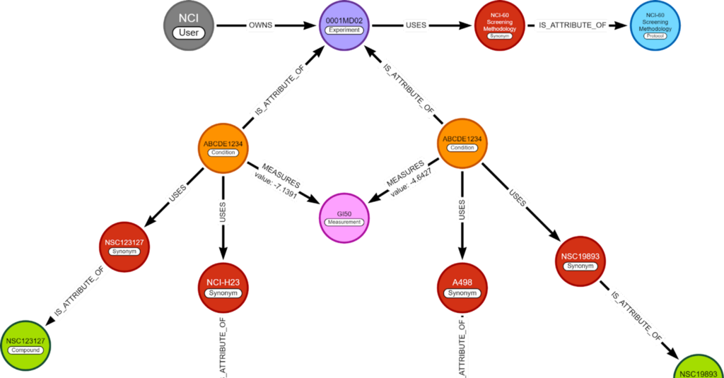
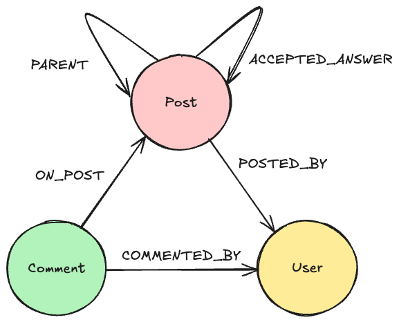
The Graph
The graph I made previously holds the experiments, their conditions, their measurements, and all variables used. This is done with the idea it can be extended later with different kinds of experiments.
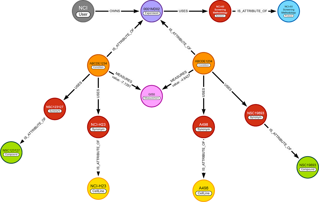
In this blog, I only care about 2 nodes, (chemical) compounds and cell lines, and 1 relationship, GI50. This means the whole graph can be simplified to this.
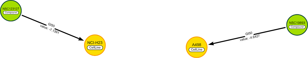
I will use the simplified graph to explain most of the logic behind the algorithm, but the queries are written for the complete graph.
Collaborative Filtering
Collaborative filtering works on the premise that “If 2 people/chemicals agree 10 out of 10 times, they will most likely also agree the 11th time”. Moshanin’s GIF explains it very clearly.

The prediction consists of 2 steps:
- Finding similar users/chemicals
- Voting between these similar ones on missing link
Finding Similar Chemicals
The relation between a chemical and a cell is non-binary. This means we need to take numbers into account to calculate the ‘difference score’.
To solve this we take the difference for each shared cell and average this.
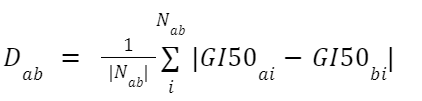
- Where Dab is the difference between chemicals a and b
- Nab is the list of all cells lines that chemicals a and b have in common
- GI50ai is the concentration of chemical a, needed for a 50% Growth Inhibition of cell line i
For example, we have 2 chemicals with 3 cell lines in common.
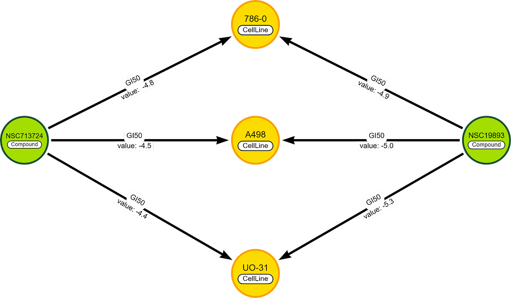
To score the difference between these chemicals, we take the GI50 values (on the relationships) and we solve the formula:
⅓ * (|-4.8 — -4.9| + |-4.5 — -5.0| + |-4.4 — -5.3|) =0.5
Voting
We search for the 25 chemicals with the lowest difference and make sure all of these have GI50 value with the cell line of interest.
Next up is the voting, many complex methods can be used. However, a simple method can already be effective; we take the average.
Implementing It
All code can be found here. I ran a Pandas implementation next to it to double-check my work.
There will be a small difference between Pandas and Cypher implementations because not all measurements are in the graph (see detailed blog for why).
Given the full query is a lot, I will build it up step by step.
GI50 Per Cell Line
The full graph shown earlier is a bit too complex for our needs. So we want 1 value between every cell line and chemical. If we find multiple values, we average them.
MATCH (org_chem:Synonym {pubChemSynId: “176dde90cc9dd83eed129de11b203b03”})
MATCH (gi50:Measurement {name: “GI50”})

MATCH (cell:CellLine)<-[:USES]-(c:Condition)-[:USES]->(org_chem)
MATCH (c)-[m:MEASURES]->(gi50)

WITH DISTINCT cell, avg(toFloat(m.value)) as values1
RETURN DISTINCT cell.name, values1
This results in an average GI50 value for 74 cell lines that are tested with chemical NSC 19893.
{‘cell.name’: ‘NCI-H23’, ‘values1’: -4.914398316498304}
{‘cell.name’: ‘NCI-H226’, ‘values1’: -3.5967323114653547}
…
{‘cell.name’: ‘A 172’, ‘values1’: -5.0341}
{‘cell.name’: ‘U87’, ‘values1’: -5.5868}
Compare 2 Chemicals
If we repeat the previous step on a second chemical (chemical B) we can calculate the difference. Here we are going to make use of the fact we already know what cell lines are connected to chemical A.
// Match to chemical A
MATCH (org_chem:Synonym {pubChemSynId: “176dde90cc9dd83eed129de11b203b03”})
MATCH (gi50:Measurement {name: “GI50”})

// Find all cell lines connected to chemical A
MATCH (cell:CellLine)<-[:USES]-(c:Condition)-[:USES]->(org_chem)
MATCH (c)-[m:MEASURES]->(gi50)

// If multiple GI50 values are know for chemical A to a cell line
// Take the the average
WITH DISTINCT cell, avg(toFloat(m.value)) as values1, gi50

// Match chemical B
MATCH (chem:Synonym {pubChemSynId: “1d75798754df81c782e805287ff7ef83”})

// Find what cell lines are connected to chemical A, also connect to chemical B
MATCH (cell)<-[:USES]-(c:Condition)-[:USES]->(chem)
MATCH (c)-[m2:MEASURES]->(gi50)

// If multiple GI50 values are know for chemical B to a cell line
// Take the the average
// Then take the difference with chemical A
WITH DISTINCT cell as cell2, abs(avg(toFloat(m2.value)) — values1) as difference, chem

// Each row has 1 cell with difference of GI50 between chemical A and B
// Average all differences
RETURN DISTINCT chem.name, avg(difference) as dist, count(difference) as num_cells
This results in a difference of ~0.53652 with 59 cell lines in common.
If we do the same with Pandas we get a difference score of ~0.53651 with also 59 cell lines in common. This shows they are close enough to each other.
Compare to All Chemicals
This query is fine if I want to compare 2 known chemicals, but I want to find the most similar chemicals of all known chemicals. To do this we remove the second chemical match and search for every chemical that shares a cell line with chemical A. To do this efficiently a call {sub query} is used. This way the subquery is called per cell line, speeding up the total query.
The rest is still the same but now a difference is given for every chemical to chemical A.
MATCH (org_chem:Synonym {pubChemSynId: “176dde90cc9dd83eed129de11b203b03”})
MATCH (gi50:Measurement {name: “GI50”})

MATCH (cell:CellLine)<-[:USES]-(c:Condition)-[:USES]->(org_chem)
MATCH (c)-[m:MEASURES]->(gi50)

WITH DISTINCT cell, avg(toFloat(m.value)) as values1, org_chem, gi50

CALL {
WITH cell, gi50, values1

MATCH (cell)<-[:USES]-(c:Condition)-[:USES]->(chem:Synonym)
MATCH (c)-[m2:MEASURES]->(gi50)

RETURN abs(avg(toFloat(m2.value)) — values1) as distance, chem
}

RETURN DISTINCT chem.name, avg(distance) as avg_dist, count(distance) as num_cell ORDER BY avg_dist limit 25
The top result will not shock you, ‘nsc19893’ looks most like ‘nsc19893’.
{‘chem.name’: ‘nsc19893’, ‘avg_dist’: 3.4386907735687276e-15, ‘num_cell’: 74}
{‘chem.name’: ‘nsc-684405’, ‘avg_dist’: 0.3018711839192636, ‘num_cell’: 60}
{‘chem.name’: ‘nsc-361605’, ‘avg_dist’: 0.3177947681672626, ‘num_cell’: 49}
{‘chem.name’: ‘nsc-628083’, ‘avg_dist’: 0.33545731366684184, ‘num_cell’: 60}
{‘chem.name’: ‘nsc-618093’, ‘avg_dist’: 0.3451951788719919, ‘num_cell’: 60}
{‘chem.name’: ‘nsc-613493’, ‘avg_dist’: 0.35390246003660175, ‘num_cell’: 50}
{‘chem.name’: ‘nsc628537’, ‘avg_dist’: 0.3781293960020346, ‘num_cell’: 46}
{‘chem.name’: ‘nsc-785594’, ‘avg_dist’: 0.3781573653571885, ‘num_cell’: 60}
{‘chem.name’: ‘nsc-628081’, ‘avg_dist’: 0.39269238426318265, ‘num_cell’: 60}
{‘chem.name’: ‘nsc-625429’, ‘avg_dist’: 0.4004440031716282, ‘num_cell’: 48}
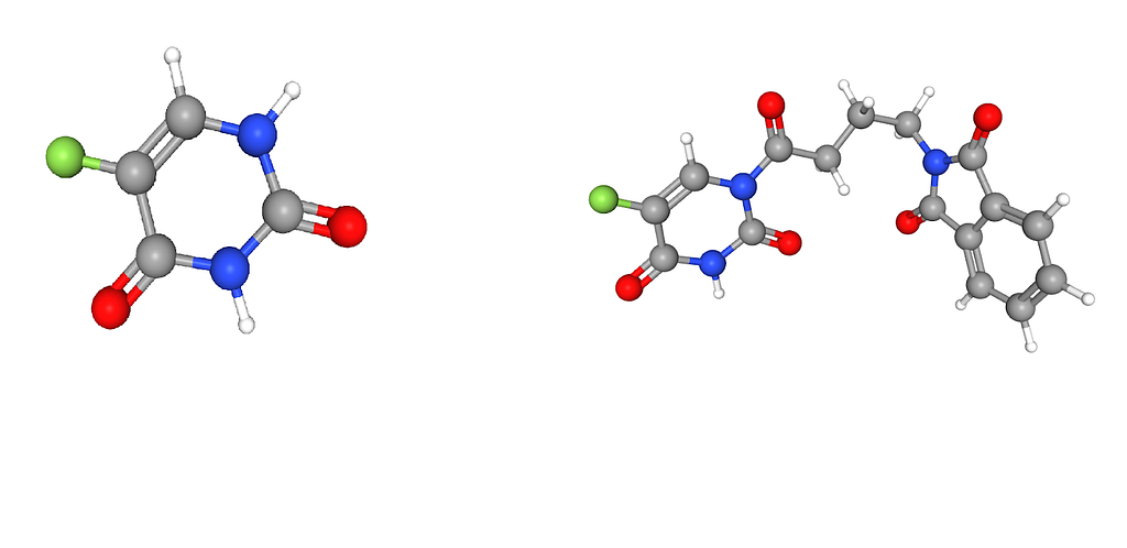
If we look up the chemical structure of NSC 19893 and NSC 684405 we see something interesting. The full structure of NSC 19893 can be found with NSC 684405. And the same is true for NSC 361605 and NSC 628083. Meaning the top 3 (that I checked) all have the same molecular structure as the chemical we compare against.
Making a Prediction
To make a prediction 3 updates need to happen:
1) Remove the cell line of interest from the collaborative filtering
Let’s say we want to predict the GI50 of chemical NSC 19893 on cell line HCT-15. We do not want to take HCT-15 into account with collaborative filtering. This is because I want to use this interaction as validation.
2) Only select chemicals with a known reaction to the cell line of interest
If a chemical does not have a known GI50 with the cell line of interest, it cannot help us make a prediction. So we ignore it.
3) Remove NSC 19893 from the predicted chemicals
Predicting yourself is just stupid.
// To still have a limit for the chemical we wrap the chemical matching in a call sub query
CALL{
MATCH (the_cell:CellLine {name: “HCT-15”})
MATCH (org_chem:Synonym {pubChemSynId: “176dde90cc9dd83eed129de11b203b03”})
MATCH (gi50:Measurement {name: “GI50”})

MATCH (cell:CellLine)<-[:USES]-(c:Condition)-[:USES]->(org_chem)
WHERE cell <> the_cell // 1)

MATCH (c)-[m:MEASURES]->(gi50)
WITH DISTINCT cell, avg(toFloat(m.value)) as values1, org_chem, gi50, the_cell

CALL {
WITH cell, gi50, values1, org_chem, the_cell
MATCH (cell)<-[:USES]-(c:Condition)-[:USES]->(chem:Synonym)
WHERE exists((chem)<-[:USES]-(:Condition)-[:USES]->(the_cell)) AND chem <> org_chem // 2) & 3)

MATCH (c)-[m2:MEASURES]->(gi50)
RETURN abs(avg(toFloat(m2.value)) — values1) as difference, chem
}

WITH DISTINCT chem, avg(difference) as avg_diff, count(difference) as num_cell
RETURN chem, avg_diff, num_cell ORDER BY avg_diff limit 25
}

// Get all reactions to cell line of interest of the 25 most similar chemicals
MATCH (the_cell)<-[:USES]-(c:Condition)-[:USES]->(chem)
MATCH (c)-[m3:MEASURES]->(gi50)

// Take the average of the 25 GI50
// We also return all values just for some analysis
WITH DISTINCT chem, avg(toFloat(m3.value)) as avg_values
RETURN avg(avg_values) as prediction, collect(avg_values) as all_values
This gives us
{‘prediction’: -4.637486125715776, ‘all_values’: [-4.727294017094016, -4.668238738738738, -4.538984496124033, -4.522523228346455, -4.5537044642857145, -4.714266037735851, -4.592720720720721, -4.5019374407582955, -4.436698214285715, -4.610763461538461, -4.541042553191488, -4.65542857142857, -4.67053893129771, -4.45142962962963, -4.965887826086957, -4.737043181818183, -4.601286440677966, -4.758097727272728, -4.699171428571429, -4.734895238095239, -4.684224, -4.787217241379309, -4.521838461538462, -4.59928888888889, -4.66263220338983]}
Validation
Complete validation is not the goal of this blog. However, I do want to give an idea that there is merit in the idea.
NSC 19893 on cell line HCT-15 has 1812 GI50 measurements, with an average of -5.24.
The 25 chemicals close to NSC 19893 predicted an average of -4.64.
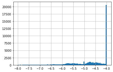
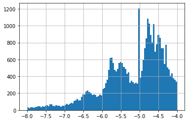
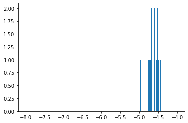
A difference of -0.6 is not a lot if we look at all GI50 on cell line HCT-15, these go from -8 to -4 (see histogram 1). A value of -4 is special given it is often the higher concentration tested. If a concentration of -4 did NOT result in a 50% Growth Inhibition, -4 is noted down. This means most of these have a true GI50 greater than -4 (see histogram 2 for -4 excluded).
None of our top 25 predictions had -4, which is a good sign. Our predictions were in a much smaller range than all HCT-15 GI50 (see histograms 2 & 3).
Using a graph recommendation algorithm for predicting chemical—cell interaction was originally published in Neo4j Developer Blog on Medium, where people are continuing the conversation by highlighting and responding to this story.
Share Article


Explore
Related Articles


How to Improve Multi-Hop Reasoning With Knowledge Graphs and LLMs