Making Sense of News, the Knowledge Graph Way

Graph ML and GenAI Research, Neo4j
17 min read
How to combine Named Entity Linking with Wikipedia data enrichment to analyze the internet news.
A wealth of information is being produced every day on the internet. Understanding the news and other content-generating websites is becoming increasingly crucial to successfully run a business. It can help you spot opportunities, generate new leads, or provide indicators about the economy.
In this blog post, I want to show you how you can create a news monitoring data pipeline that combines natural language processing (NLP) and knowledge graph technologies.
The data pipeline consists of three parts. In the first part, we scrape articles from an Internet provider of news. Next, we run the articles through an NLP pipeline and store results in the form of a knowledge graph. In the last part of the data pipeline, we enrich our knowledge with information from the WikiData API. To demonstrate the benefits of using a knowledge graph to store the information from the data pipeline, we perform simple network analysis and try to find insights.
Agenda
- Scraping internet news
- Entity linking with Wikifier
- Wikipedia data enrichment
- Network analysis
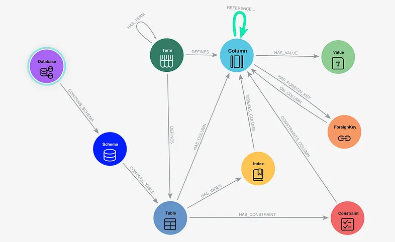
Graph Model
We use Neo4j to store our knowledge graph. If you want to follow along with this blog post, you need to download Neo4j and install both the APOC and Graph Data Science libraries. All the code is available on GitHub as well.
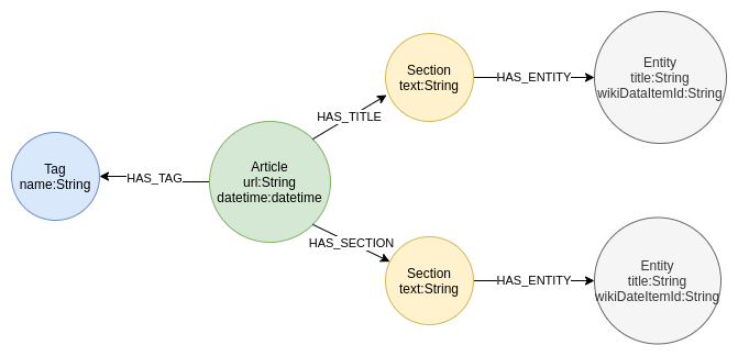
Our graph data model consists of articles and their tags. Each article has many sections of text. Once we run the section text through the NLP pipeline, we extract and store mentioned entities back to our graph.
We start by defining unique constraints for our graph.
Uniqueness constraints are used to ensure data integrity, as well as to optimize Cypher query performance.
CREATE CONSTRAINT IF NOT EXISTS ON (a:Article) ASSERT a.url IS UNIQUE;
CREATE CONSTRAINT IF NOT EXISTS ON (e:Entity) ASSERT e.wikiDataItemId is UNIQUE;
CREATE CONSTRAINT IF NOT EXISTS ON (t:Tag) ASSERT t.name is UNIQUE;
Internet News Scraping
Next, we scrape the CNET news portal. I have chosen the CNET portal because it has the most consistent HTML structure, making it easier to demonstrate the data pipeline concept without focusing on the scraping element. We use theapoc.load.html procedure for the HTML scraping. It uses jsoup under the hood. Find more information in the documentation.
First, we iterate over popular topics and store the link of the last dozen of articles for each topic in Neo4j.
CALL apoc.load.html("https://www.cnet.com/news/",
  {topics:"div.tag-listing > ul > li > a"}) YIELD value
UNWIND value.topics as topic
WITH "https://www.cnet.com" + topic.attributes.href as link
CALL apoc.load.html(link, {article:"div.row.asset > div > a"}) YIELD value
UNWIND value.article as article
WITH distinct "https://www.cnet.com" + article.attributes.href as article_link
MERGE (a:Article{url:article_link});
Now that we have the links to the articles, we can scrape their content as well as their tags and publishing date. We store the results according to the graph schema we defined in the previous section.
MATCH (a:Article)
CALL apoc.load.html(a.url,
{date:"time", title:"h1.speakableText", text:"div.article-main-body > p", tags: "div.tagList > a"}) YIELD value
SET a.datetime = datetime(value.date[0].attributes.datetime)
FOREACH (_ IN CASE WHEN value.title[0].text IS NOT NULL THEN [true] ELSE [] END |
           CREATE (a)-[:HAS_TITLE]->(:Section{text:value.title[0].text})
)
FOREACH (t in value.tags |
  MERGE (tag:Tag{name:t.text}) MERGE (a)-[:HAS_TAG]->(tag)
)
WITH a, value.text as texts
UNWIND texts as row
WITH a,row.text as text
WHERE text IS NOT NULL
CREATE (a)-[:HAS_SECTION]->(:Section{text:text});
I did not want to complicate the Cypher query that stores the results of the articles even more, so we must perform a minor cleanup of tags before we continue.
MATCH (n:Tag)
WHERE n.name CONTAINS "Notification"
DETACH DELETE n;
Let’s evaluate our scraping process and look at how many of the articles have been successfully scraped.
MATCH (a:Article)
RETURN exists((a)-[:HAS_SECTION]->()) as scraped_articles,
       count(*) as count
In my case, I have successfully collected the information for 245 articles. Unless you have a time machine, you won’t be able to recreate this analysis identically. I have scraped the website on the 30th of January 2021, and you will probably do it later. I have prepared most of the analysis queries generically, so they work regardless of the date you choose to scrape the news.
Let’s also examine the most frequent tags of the articles.
MATCH (n:Tag)
RETURN n.name as tag, size((n)<-[:HAS_TAG]-()) as articles
ORDER BY articles DESC
LIMIT 10
Here are the results:
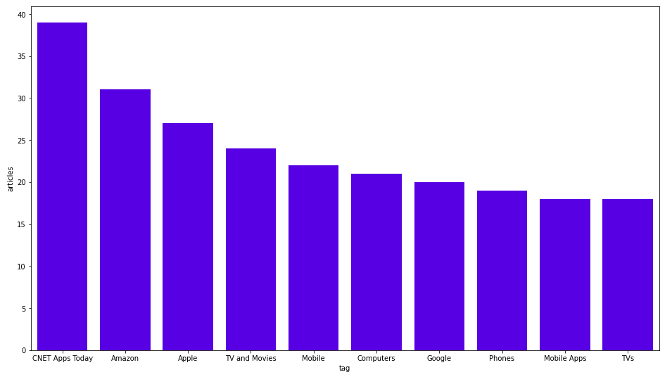
All charts in this blog post are made using the Seaborn library. CNET Apps Today is the most frequent tag. I think that’s just a generic tag for daily news. We can observe that they have custom tags for various big companies such as Amazon, Apple, and Google.
Named Entity Linking: Wikification
In my previous blog post, we have already covered the Named Entity Recognition techniques to create a knowledge graph. Here, we will take it up a notch and delve into Named Entity Linking.
First of all, what exactly is Named Entity Linking?
Named Entity Linking is an upgrade to the entity recognition technique. It starts by recognizing all the entities in the text. Once it finishes the named entity recognition process, it tries to link those entities to a target knowledge base. Usually, the target knowledge bases are Wikipedia or DBpedia, but there are other knowledge bases out there as well.
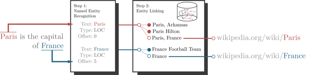
In the above example, we can observe that the named entity recognition process recognized Paris as an entity. The next step is to link it to a target entity in a knowledge base. Here, it uses Wikipedia as the target knowledge base. This is also known as the Wikification process.
The Entity Linking process is a bit tricky as we can see that many entities exist in Wikipedia that have Paris in their title. So, as a part of the Entity Linking process, the NLP model also does the entity disambiguation.
There are a dozen Entity Linking models out there. Some of them are:
- https://wikifier.org/
- https://www.mpi-inf.mpg.de/departments/databases-and-information-systems/research/ambiverse-nlu/aida
- https://github.com/informagi/REL
- https://github.com/facebookresearch/BLINK
I am from Slovenia, so my biased decision is to use the Slovenian solution Wikifier [1]. They don’t actually offer their NLP model, but they have a free-to-use API endpoint. All you have to do is to register. They don’t even want your password or email, which is nice of them.
The Wikifier supports more than 100 languages. It also features some parameters you can use to fine-tune the results. I have noticed that the most dominant parameter is the pageRankSqThreshold parameter, which you can use to optimize either recall or accuracy of the model.
If we run the above example through the Wikifier API, we get the following results:
We can observe that Wikifier API returned three entities and their corresponding Wikipedia URL as well as WikiData item id. We use the WikiData item id as a unique identifier for storing them back to Neo4j.
The APOC library has the apoc.load.json procedure, which you can use to retrieve results from any API endpoint. If you are dealing with a larger amount of data, you will want to use the apoc.periodic.iterate procedure for batching purposes.
If we put it all together, the following Cypher query fetches the annotation results for each section from the API endpoint and stores the results in Neo4j.
CALL apoc.periodic.iterate('
 MATCH (s:Section) RETURN s
 ','
 WITH s, "https://www.wikifier.org/annotate-article?" +
        "text=" + apoc.text.urlencode(s.text) + "&" +
        "lang=en&" +
        "pageRankSqThreshold=0.80&" +
        "applyPageRankSqThreshold=true&" +
        "nTopDfValuesToIgnore=200&" +
        "nWordsToIgnoreFromList=200&" +
        "minLinkFrequency=100&" +
        "maxMentionEntropy=10&" +
        "wikiDataClasses=false&" +
        "wikiDataClassIds=false&" +
        "userKey=" + $userKey as url
CALL apoc.load.json(url) YIELD value
UNWIND value.annotations as annotation
MERGE (e:Entity{wikiDataItemId:annotation.wikiDataItemId})
ON CREATE SET e.title = annotation.title, e.url = annotation.url
MERGE (s)-[:HAS_ENTITY]->(e)',
{batchSize:100, params: {userKey:$user_key}})
The Named Entity Linking process takes a couple of minutes. We can now check the most frequently mentioned entities.
MATCH (e:Entity)
RETURN e.title, size((e)<--()) as mentions
ORDER BY mentions DESC LIMIT 10;
Here are the results:
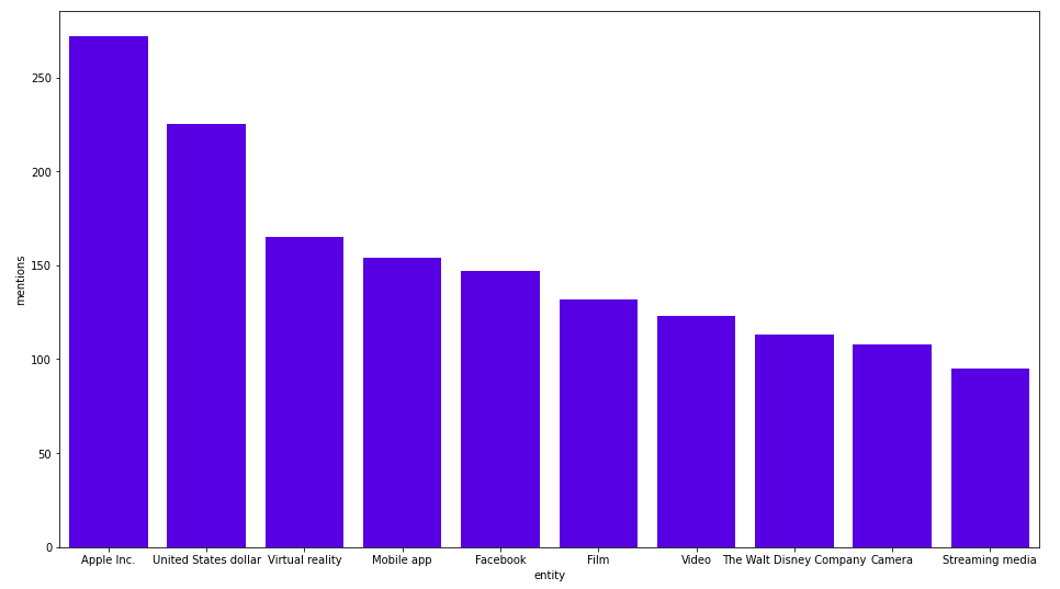
Apple Inc. is the most frequently mentioned entity. I am guessing that all dollar signs or USD mentions get linked to the United States dollar. We can also examine the most frequently-mentioned-by-article tags.
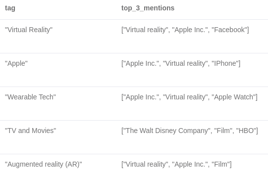
MATCH (e:Entity)<-[:HAS_ENTITY]-()<-[:HAS_SECTION]-()-[:HAS_TAG]->(tag)
WITH tag.name as tag, e.title as title, count(*) as mentions
ORDER BY mentions DESC
RETURN tag, collect(title)[..3] as top_3_mentions
LIMIT 5;
Here are the results:
WikiData Enrichment
A bonus to using the Wikification process is that we have the WikiData item id of our entities. This makes it very easy for us to scrape the WikiData API for additional information.
Let’s say we want to define all business and person entities. We will fetch the entity classes from WikiData API and use that information to group the entities. Again we will use the apoc.load.json procedure to retrieve the response from an API endpoint.
MATCH (e:Entity)
// Prepare a SparQL query
WITH 'SELECT *
      WHERE{
        ?item rdfs:label ?name .
        filter (?item = wd:' + e.wikiDataItemId + ')
        filter (lang(?name) = "en" ) .
      OPTIONAL{
        ?item wdt:P31 [rdfs:label ?class] .
        filter (lang(?class)="en")
      }}' AS sparql, e
// make a request to Wikidata
CALL apoc.load.jsonParams(
    "https://query.wikidata.org/sparql?query=" +
    apoc.text.urlencode(sparql),
     { Accept: "application/sparql-results+json"}, null)
YIELD value
UNWIND value['results']['bindings'] as row
FOREACH(ignoreme in case when row['class'] is not null then [1] else [] end |
        MERGE (c:Class{name:row['class']['value']})
        MERGE (e)-[:INSTANCE_OF]->(c));
We continue by inspecting the most frequent classes of the entities.
MATCH (c:Class)
RETURN c.name as class, size((c)<--()) as count
ORDER BY count DESC LIMIT 5;
Here are the results:
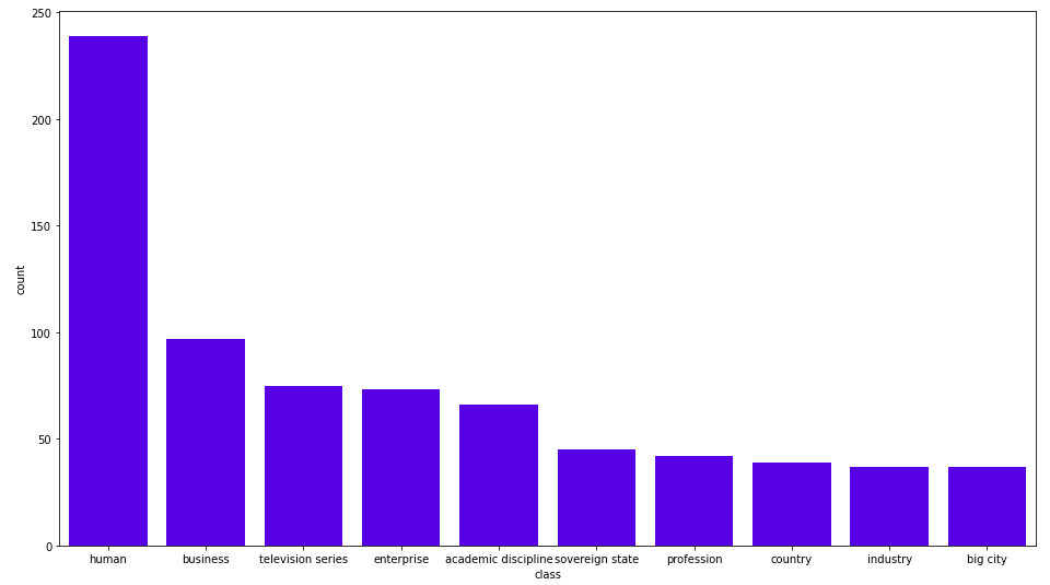
The Wikification process found almost 250 human entities and 100 business entities. We assign a secondary label to Person and Business entities to simplify our further Cypher queries.
MATCH (e:Entity)-[:INSTANCE_OF]->(c:Class)
WHERE c.name in ["human"]
SET e:Person;
MATCH (e:Entity)-[:INSTANCE_OF]->(c:Class)
WHERE c.name in ["business", "enterprise"]
SET e:Business;
With the added secondary label, we can now easily examine the most frequently-mentioned business entities.
MATCH (b:Business)
RETURN b.title as business, size((b)<-[:HAS_ENTITY]-()) as mentions
ORDER BY mentions DESC
LIMIT 10
Here are the results:
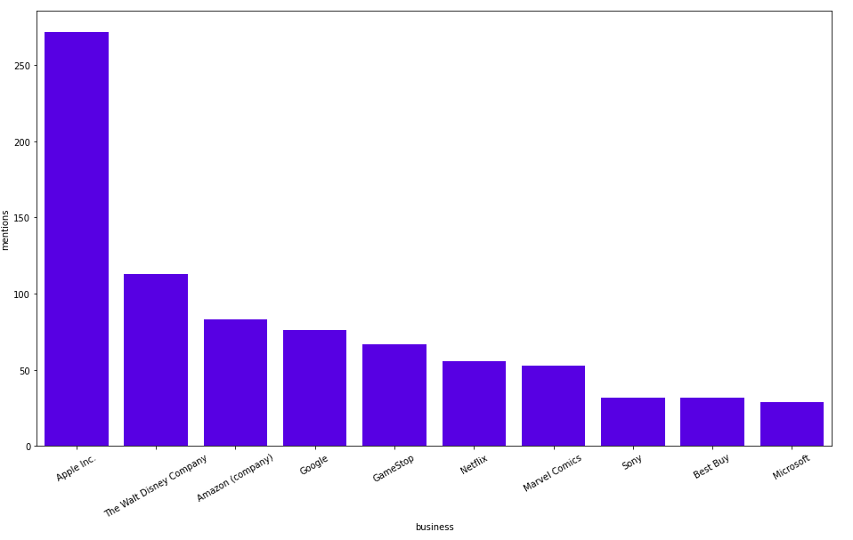
We already knew that Apple and Amazon were discussed a lot. Some of you already know that this was an exciting week on the stock market, as we can see lots of mentions of GameStop.
Just because we can, let’s also fetch the industries of the business entities from the WikiData API.
MATCH (e:Business)
// Prepare a SparQL query
WITH 'SELECT *
      WHERE{
        ?item rdfs:label ?name .
        filter (?item = wd:' + e.wikiDataItemId + ')
        filter (lang(?name) = "en" ) .
      OPTIONAL{
        ?item wdt:P452 [rdfs:label ?industry] .
        filter (lang(?industry)="en")
      }}' AS sparql, e
// make a request to Wikidata
CALL apoc.load.jsonParams(
    "https://query.wikidata.org/sparql?query=" +
    apoc.text.urlencode(sparql),
     { Accept: "application/sparql-results+json"}, null)
YIELD value
UNWIND value['results']['bindings'] as row
FOREACH(ignoreme in case when row['industry'] is not null then [1] else [] end |
        MERGE (i:Industry{name:row['industry']['value']})
        MERGE (e)-[:PART_OF_INDUSTRY]->(i));
Exploratory Graph Analysis
Our data pipeline ingestion is complete. Now we can have some fun and explore our knowledge graph. First, we will examine the most co-occurrent entities of the most frequently-mentioned entity, which is Apple Inc. in my case.
MATCH (b:Business)
WITH b, size((b)<-[:HAS_ENTITY]-()) as mentions
ORDER BY mentions DESC
LIMIT 1
MATCH (other_entities)<-[:HAS_ENTITY]-()-[:HAS_ENTITY]->(b)
RETURN other_entities.title as entity, count(*) as count
ORDER BY count DESC LIMIT 10;
Here are the results:
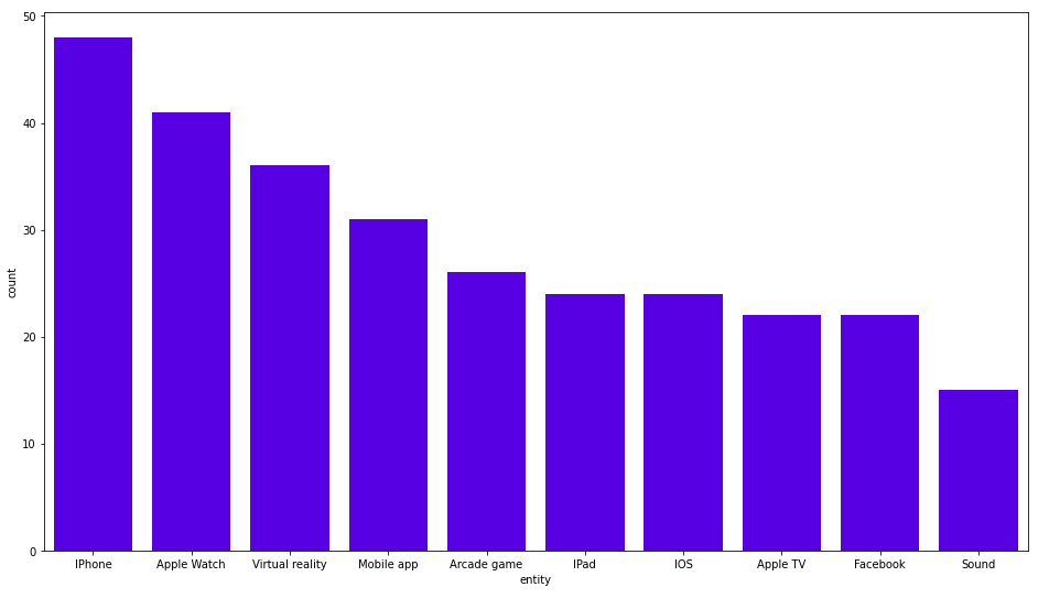
Nothing spectacular here. Apple Inc. appears in sections where iPhone, Apple Watch, and VR are also mentioned. We can look at some more exciting news. I was searching for any relevant tags of articles that might be interesting.
CNET has many specific tags, but the Stock Market tag stood out as more broad and very relevant in these times. Let’s check the most frequently-mentioned industries in the Stock Market category of articles.
MATCH (t:Tag)<-[:HAS_TAG]-()-[:HAS_SECTION]->()-[:HAS_ENTITY]->(entity:Business)-[:PART_OF_INDUSTRY]->(industry)
WHERE t.name = "Stock Market"
RETURN industry.name as industry, count(*) as mentions
ORDER BY mentions DESC
LIMIT 10
Here are the results:
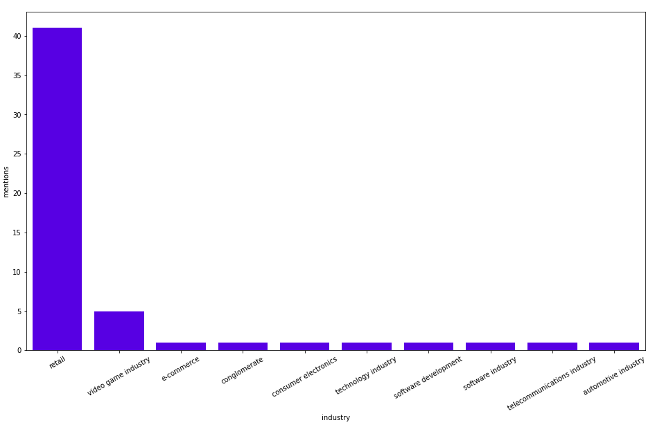
Retail is by far the most mentioned, next is the video game industry, and then some other industries that are mentioned only once. Next, we will check the most mentioned businesses or persons in the Stock Market category.
MATCH (t:Tag)<-[:HAS_TAG]-()-[:HAS_SECTION]->()-[:HAS_ENTITY]->(entity)
WHERE t.name = "Stock Market" AND (entity:Person OR entity:Business)
RETURN entity.title as entity, count(*) as mentions
ORDER BY mentions DESC
LIMIT 10
Here are the results:
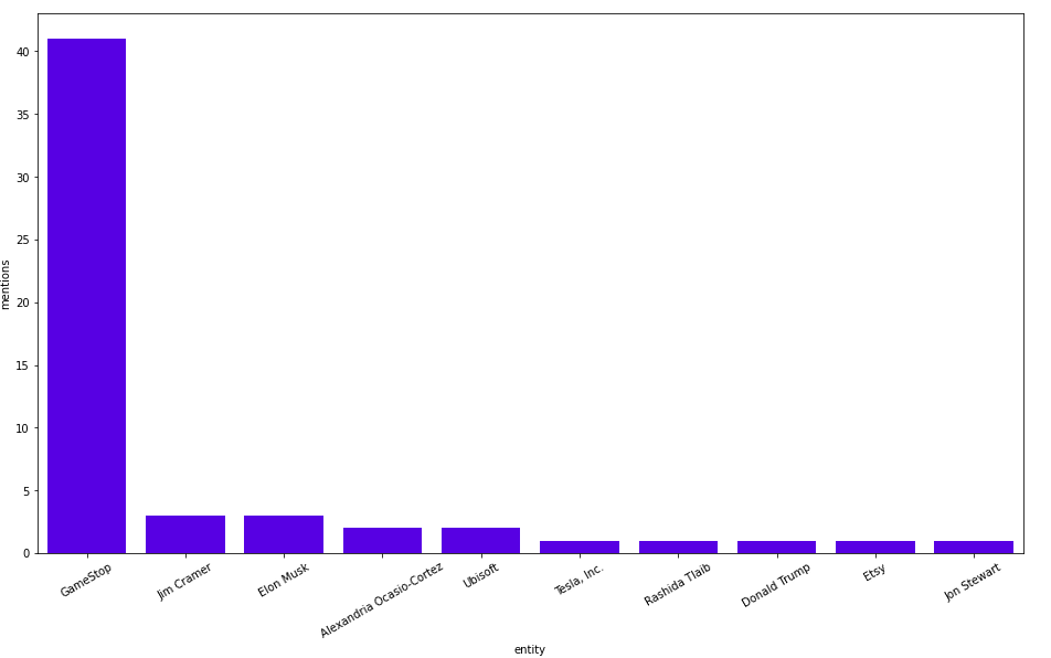
Okay, so GameStop is huge this weekend with more than 40 mentions. Very far behind are Jim Cramer, Elon Musk, and Alexandria Ocasio-Cortez. Let’s try to understand why GameStop is so huge by looking at the co-occurring entities.
MATCH (b:Business{title:"GameStop"})<-[:HAS_ENTITY]-()-[:HAS_ENTITY]->(other_entity)
RETURN other_entity.title as co_occurent_entity, count(*) as mentions
ORDER BY mentions DESC
LIMIT 10
Here are the results:
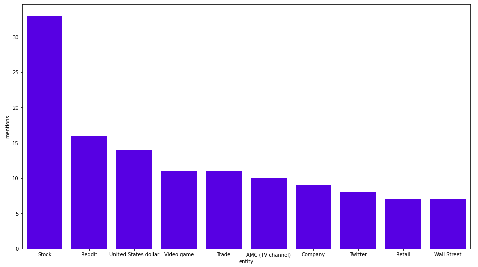
The most frequently-mentioned entities in the same section as GameStop are Stock, Reddit, and US dollar. If you look at the news you might see that the results make sense. I would venture a guess that AMC (TV channel) was wrongly identified and should probably be the AMC Theaters company.
There will always be some mistakes in the NLP process. We can filter the results a bit and look for the most co-occurring person or business entities of GameStop.
MATCH (b:Business{title:"GameStop"})<-[:HAS_ENTITY]-()-[:HAS_ENTITY]->(other_entity:Person)
RETURN other_entity.title as co_occurent_entity, count(*) as mentions
ORDER BY mentions DESC
LIMIT 10
Here are the results:
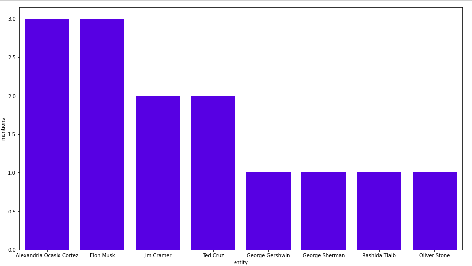
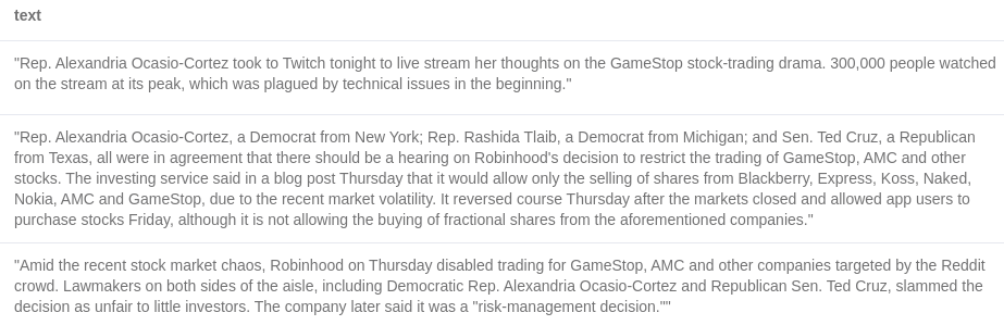
Alexandria Ocasio-Cortez(AOC) and Elon Musk each appear in three sections with GameStop. Let’s examine the text where AOC co-occurs with GameStop.
MATCH (b:Business{title:"GameStop"})<-[:HAS_ENTITY]-(section)-[:HAS_ENTITY]->(p:Person{title:"Alexandria Ocasio-Cortez"})
RETURN section.text as text
Here are the results:
Graph Data Science
So far, we have only done a couple of aggregations using the Cypher query language. As we are utilizing a knowledge graph to store our information, let’s execute some graph algorithms on it. Neo4j Graph Data Science library is a plugin for Neo4j that currently has more than 50 graph algorithms available. The algorithms range from community detection and centrality to node embedding and graph neural network categories.
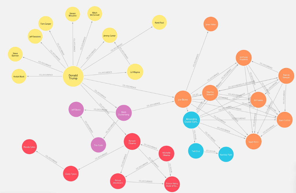
We have already inspected some co-occurring entities so far. Next, we infer a co-occurrence network of persons within our knowledge graph. This process basically translates indirect relationships, where two entities are mentioned in the same section, to a direct relationship between those two entities. This diagram might help you understand the process.
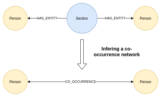
The Cypher query for inferring the person co-occurrence network is:
MATCH (s:Person)<-[:HAS_ENTITY]-()-[:HAS_ENTITY]->(t:Person)
WHERE id(s) < id(t)
WITH s,t, count(*) as weight
MERGE (s)-[c:CO_OCCURENCE]-(t)
SET c.weight = weight
The first graph algorithm we use is the Weakly Connected Components algorithm. It is used to identify disconnected components or islands within the network.
CALL gds.wcc.write({
    nodeProjection:'Person',
    relationshipProjection:'CO_OCCURENCE',
    writeProperty:'wcc'})
YIELD componentCount, componentDistribution
Here are the results:
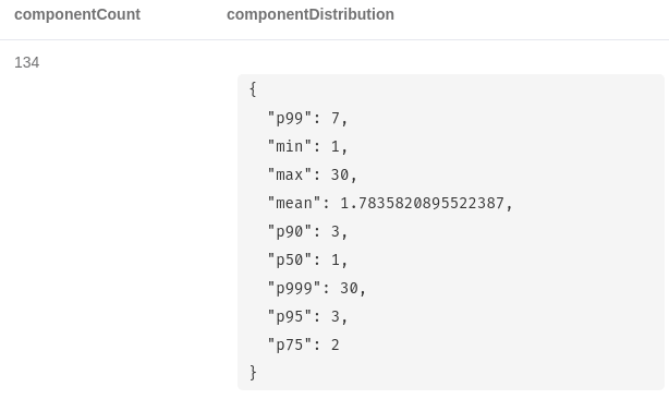
The algorithm found 134 disconnected components within our graph. The p50 value is the 50th percentile of the community size. Most of the components consist of a single node.
This implies that they don’t have any CO_OCCURENCE relationships. The largest island of nodes consists of 30 members. We mark its members with a secondary label.
MATCH (p:Person)
WITH p.wcc as wcc, collect(p) as members
ORDER BY size(members) DESC LIMIT 1
UNWIND members as member
SET member:LargestWCC
We further analyze the largest component by examining its community structure and trying to find the most central nodes. When you have a plan to run multiple algorithms on the same projected graph, it is better to use a named graph. The relationship in the co-occurrence network is treated as undirected.
CALL gds.graph.create('person-cooccurence', 'LargestWCC',
  {CO_OCCURENCE:{orientation:'UNDIRECTED'}},
  {relationshipProperties:['weight']})
First, we run the PageRank algorithm, which helps us identify the most central nodes.
CALL gds.pageRank.write('person-cooccurence', {relationshipWeightProperty:'weight', writeProperty:'pagerank'})
Next, we run the Louvain algorithm, which is a community detection algorithm.
CALL gds.louvain.write('person-cooccurence', {relationshipWeightProperty:'weight', writeProperty:'louvain'})
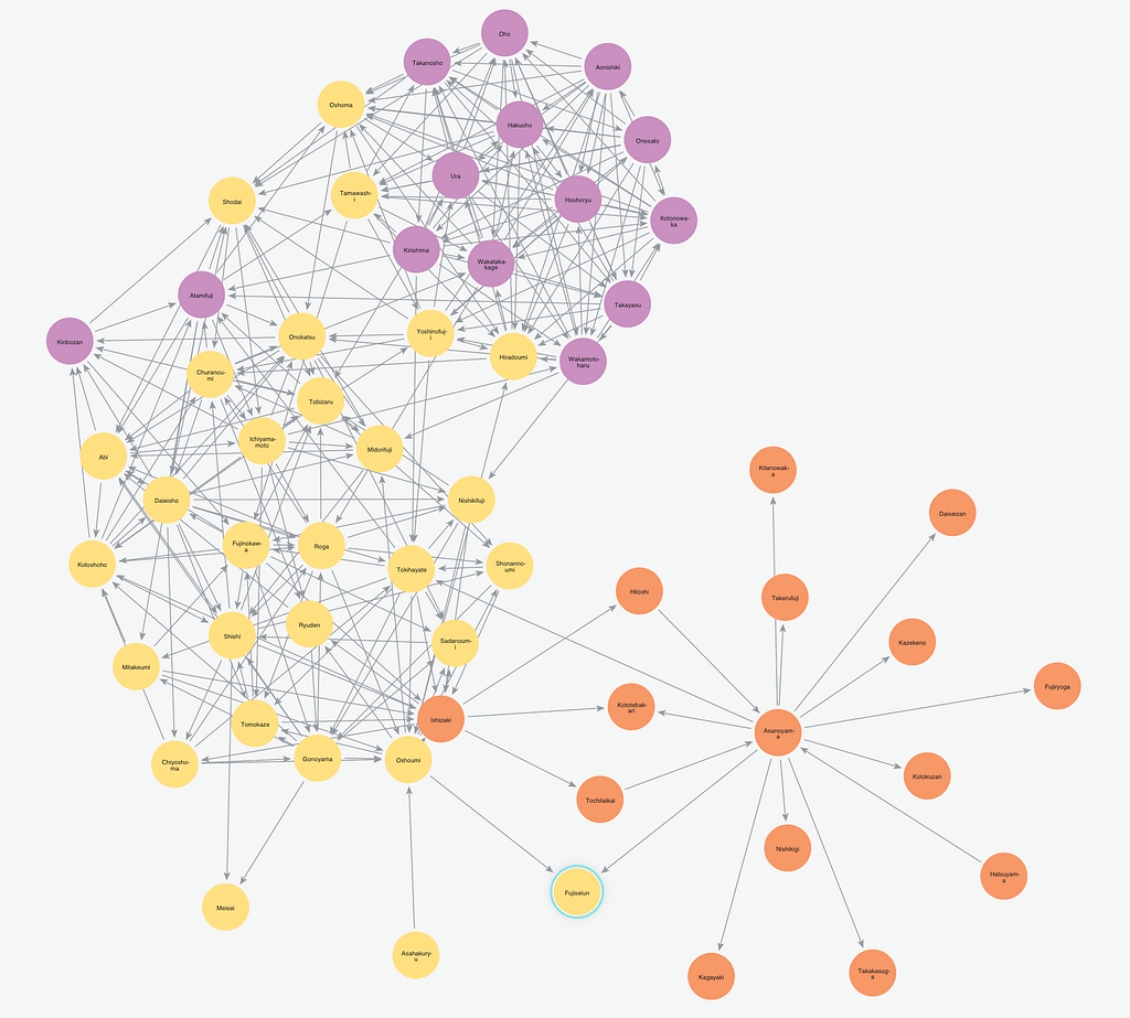
Some people say that a picture is worth a thousand words. When you are dealing with smaller networks it makes sense to create a network visualization of the results. The following visualization was created using Neo4j Bloom.
Conclusion
I really love how NLP and knowledge graphs are a perfect match. Hopefully, I have given you some ideas and pointers on how you can go about implementing your data pipeline and storing results in a form of a knowledge graph. Let me know what do you think!
As always, the code is available on GitHub.
References
[1] Janez Brank, Gregor Leban, Marko Grobelnik. Annotating Documents with Relevant Wikipedia Concepts. Proceedings of the Slovenian Conference on Data Mining and Data Warehouses (SiKDD 2017), Ljubljana, Slovenia, 9 October 2017.
Making Sense of News, the Knowledge Graph Way was originally published in Neo4j Developer Blog on Medium, where people are continuing the conversation by highlighting and responding to this story.
Share Article


Explore
Related Articles
How a Neo4j semantic layer makes your Text-to-SQL agent smarter and cheaper
Building graph-based agentic systems: Failures, fixes, and how the answer gets there — Part 2