PyNeoInstance: A user-friendly Python library for Neo4j

Senior AI Solutions Architect, Neo4j
8 min read

Introduction
PyNeoInstance was created by my Neo4j colleague Jose Alvarado-Guzman. It allows for easy loading and reading of data in a Neo4j graph by handling tasks such as driver creation and multiprocessing and supports simple configuration with YAML.
I have provided a demo GitHub repo here so you can follow along and use this as a starting point for your own projects.
Requirements
- A free Neo4j AuraDB instance
- Familiarity with Cypher Query Language
- Familiarity with Python and Notebooks
AuraDB

In order to demonstrate PyNeoInstance, we will use a freeAuraDB instance from Neo4j. Quickly set up an AuraDB instance by following the below steps.
- Follow this link to the Aura console.
- Create a free AuraDB instance (not AuraDS).
- Save the provided file containing your connection information in a safe location.
Note: Your Aura instance will be paused after 3 days of inactivity and eventually will be auto-deleted if you don’t access it.
Data
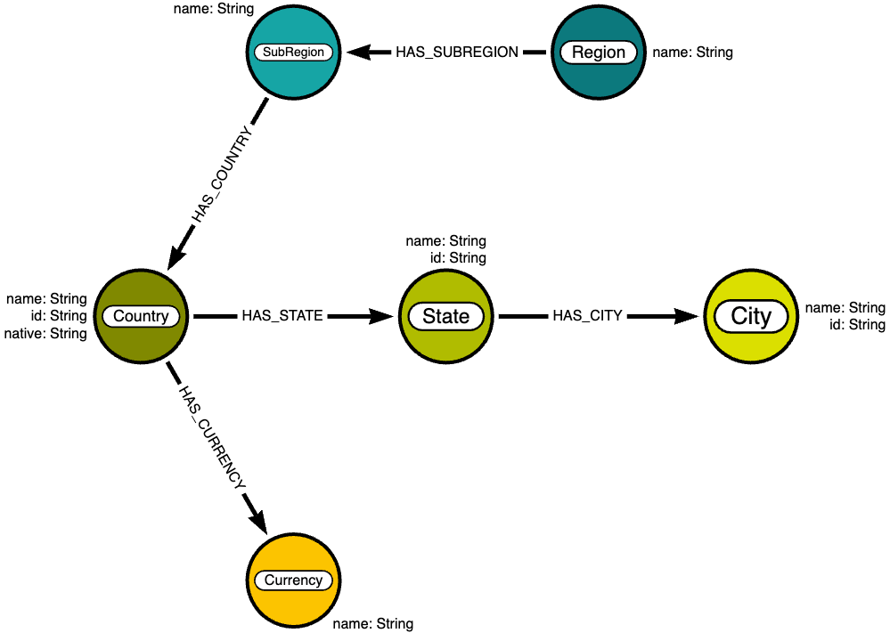
We will be using data on world countries, cities, etc, provided by mexwell via Kaggle. It is included in the provided GitHub repo or can be found here. From this, we will create a simple graph with the following data model.
Configuration
We will use a YAML file to store our project information. This includes database connection information and any read / write queries we may run. If you are following along in the repo project it is the config.yaml file.
Database info
With the file you received from Aura, replace the information in the config.yaml file with your connection information.
db_info:
  uri: bolt://localhost:7687
  database: neo4j
  user: neo4j
  password: password
Initialization queries
Next, we will explore the initializing queries. This section contains the constraints and indexes we will create before any data ingestion. These constraints greatly speed up ingestion by indexing and ensuring the uniqueness of the node properties we will be matching on.
initializing_queries:
  constraints:
    unique_country: |
      CREATE CONSTRAINT unique_country
      FOR (c:Country) REQUIRE c.id IS UNIQUE;
    unique_state: |
      CREATE CONSTRAINT unique_state
      FOR (s:State) REQUIRE s.id IS UNIQUE;
    ...
  indexes:
    ...
We don’t currently need to include additional indexes because we only need the constrained properties indexed in this example graph. If you’re adapting this file for your own project and would like to index unconstrained properties, then you can create indexes here in the following format.
indexes:
    my_index: |
      CREATE INDEX my_index
      FOR (n:Person) ON (n.name);
    my_second_index: |
      ...
Ingestion queries
Once our initializing queries are set, we can define our ingestion queries. These will be used to load data into the graph. First, we define how we will load the nodes. Each CSV we want to load will have its own YAML section, and each query must begin the lines:
with $rows as rows
unwind rows as row
This allows us to iterate over the provided Pandas DataFrame and load content into the graph. We then use MERGE commands to check if a node exists in the graph already. If it’s absent, then we create a new node.
loading_queries:
  nodes:
    countries: |
      with $rows as rows
      unwind rows as row

      merge (c:Country {id: row.iso2})
      merge (:Currency {name: row.currency})
      merge (:Region {name: row.region})
      merge (:SubRegion {name: row.subregion})

      set c.name = row.name

    states: |
      with $rows as rows
      unwind rows as row

      merge (s:State {id: row.id})

      set s.name = row.name
  ...
Note: We include the constrained properties defined above in the MERGE line.
The last part of our ingestion queries handles loading relationships into the graph. These are loaded separately from nodes to prevent locking issues and missing relationships. We must ensure that all nodes are loaded first before attempting to create relationships among them.
loading_queries:
  nodes:
  ...
  relationships:
    countries: |
      with $rows as rows
      unwind rows as row

      match (c:Country {id: row.iso2})
      match (cur:Currency {name: row.currency})
      match (r:Region {name: row.region})
      match (sr:SubRegion {name: row.subregion})

      merge (r)-[:HAS_SUBREGION]->(sr)
      merge (sr)-[:HAS_COUNTRY]->(c)
      merge (c)-[:HAS_CURRENCY]->(cur)
     ...
Here, we are using MATCH to match the nodes we’d like to connect, then using MERGE to create that relationship between the matched nodes if it doesn’t already exist.
Analysis queries
The final section of our YAML file will contain analysis queries. The results of these queries will be returned as Pandas DataFrames.
analysis_queries:
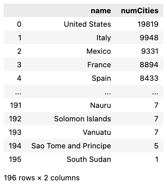
cities_per_country: |
match (co:Country)--(:State)--(ci:City)
return co.name as name,
count(ci) as numCities
order by numCities desc
Ingestion
Now, we will detail the steps taken in the provided ingest.ipynb notebook. After loading the CSV data into Pandas DataFrames, we load the YAML information into easily accessible variables.
config = load_yaml_file("config.yaml")
db_info = config['db_info']
constraints = config['initializing_queries']['constraints']
indexes = config['initializing_queries']['indexes']
node_load_queries = config['loading_queries']['nodes']
relationship_load_queries = config['loading_queries']['relationships']
We then connect to our graph…
graph = Neo4jInstance(db_info['uri'], db_info['user'], db_info['password'])
And create our constraints and indexes before moving on to ingestion.
try:
    graph.execute_write_queries(database=db_info['database'], queries=list(constraints.values()))
except Exception as e:
    print(e)
try:
    graph.execute_write_queries(database=db_info['database'], queries=list(indexes.values()))
except Exception as e:
    print(e)
Loading in parallel
PyNeoInstance supports batching and allows us to execute write queries in parallel.
Batching allows us to load our data into the graph in different transactions incrementally. Loading in batches is recommended if your DataFrames are larger than 100,000 rows.
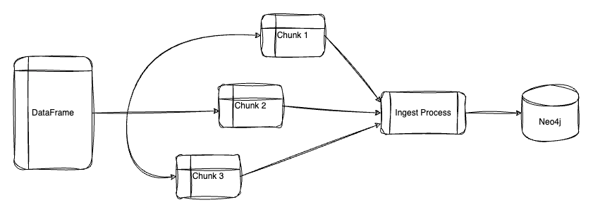
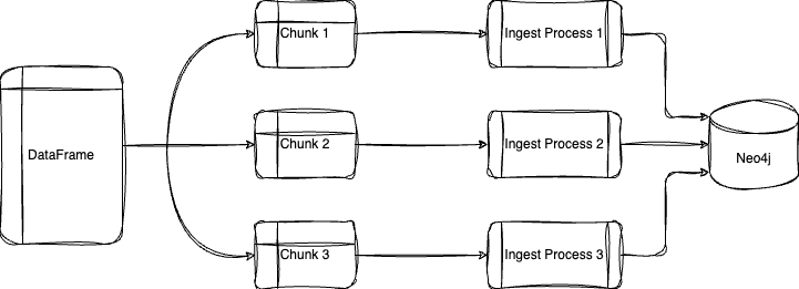
Parallel loading takes advantage of your machine’s multiprocessing capabilities to greatly decrease ingestion time. To enable this, we can set the below parameters in the method:
- parallel = True
- partitions = Number of chunks to split DataFrame into
- workers = Number of virtual CPUs used to execute query
I have also included a method that will calculate the number of partitions given a desired batch size.
def get_partition(data: pd.DataFrame, batch_size: int = 500) -> int:
    """
    Determine the data partition based on the desired batch size.
    """

    partition = int(len(data) / batch_size)
    return partition if partition > 1 else 1
Loading nodes
We load our nodes in parallel with the below code. This iterates through tuples of (DataFrame, query key) to load the data into the graph.
for data, query in list(zip([cities_df, countries_df, states_df], ['cities', 'countries', 'states'])):
    res = graph.execute_write_query_with_data(database=db_info['database'],
                                                data=data,
                                                query=node_load_queries[query],
                                                partitions=get_partition(data, batch_size=500),
                                                parallel=True,
                                                workers=2)
Note: If we leave the workers parameter empty, it will default to all available virtual CPUs on the machine.
Loading relationships
We load our relationships in a similar manner as above, except this time, we use CREATE instead of MERGE when loading some of the data. We use CREATE when we know that each row of the DataFrame we are loading contains unique relationships. If we are unsure or if we know there is duplicate data, we should use MERGE without parallel loading. In this example, we use MERGE with the countries’ data because the (Region) →(SubRegion) relationship is present multiple times.
for data, query in list(zip([cities_df, states_df], ['cities', 'states'])):
    res = graph.execute_write_query_with_data(  database=db_info['database'],
                                                data=data,
                                                query=relationship_load_queries[query],
                                                partitions=get_partition(data, batch_size=500),
                                                parallel=True,
                                                workers=2)

graph.execute_write_query_with_data(  database=db_info['database'],
                                                data=countries_df,
                                                query=relationship_load_queries["countries"],
                                                partitions=get_partition(data, batch_size=500))
Analysis
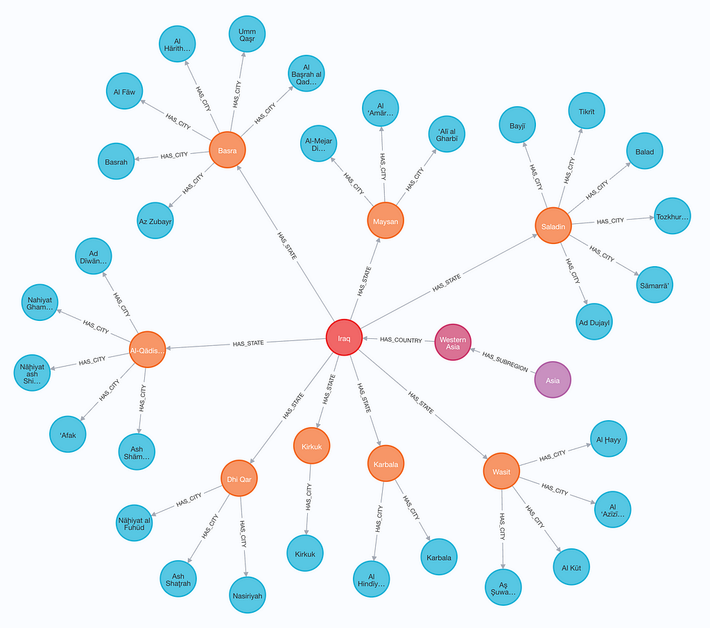
Once loaded, we can take a look at our graph. This can be done by navigating to the Aura console, opening your instance, and entering a query. The graph below is generated with the query:
match p=(:Region)--()--(:Country)--()--(:City)
return p
limit 100
Let’s load an analysis query from our config file and see the results. When we run a query, it will be returned as a Pandas DataFrame. Additional analysis query results can be found in the provided analysis.ipynb notebook.
cities_per_country = graph.execute_read_query(query=queries['cities_per_country'], database=db_info['database'])
Conclusion
We now know how to use PyNeoInstance to easily load and query a graph. The repository for this project can be found here: https://github.com/a-s-g93/pyneoinstance-tutorial. Please feel free to use its contents as a starting point for your own projects.
If you’d like to see more examples of PyNeoInstance in action, please check out my colleague Cayley Causey’s series on Scooby Doo data here: https://medium.com/@cayley.causey/loading-data-into-neo4j-using-pyneoinstance-scoobygraph-part-2-e0bd35bc0cd3
PyNeoInstance: A User-Friendly Python Library for Neo4j was originally published in Neo4j Developer Blog on Medium, where people are continuing the conversation by highlighting and responding to this story.
Share Article


Explore
Related Articles
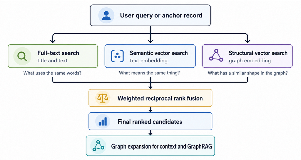
Hybrid Search in Neo4j: Full-Text, Vectors, and Graph Topology with Cypher