Knowledge Graph Generation

Consulting Engineer, Neo4j
21 min read
Strategies and methods for knowledge graph generation
Neo4j contributes to two primary components of knowledge management in the GenAI ecosystem: construction and retrieval. Ultimately, these components position Neo4j as an ideal context provider for GenAI applications. This context layer can be used for various applications, such as memory management, agent tool storage, or domain graph analytics. In this article, we’ll focus on ingestion and knowledge graph generation. This is a process by which we can create and augment a graph that connects unstructured and structured data, providing the context layer for AI applications.

A knowledge graph provides many benefits over other data stores as the context layer. With a graph, we can use structured and unstructured data, while also taking advantage of embeddings. We’re also able to perform complex filtering and traversals since relationships between entities are explicitly stored. By using graphs to build our context layer, we can implement GraphRAG retrieval patterns that aren’t possible with other data stores.
A GraphRAG method is one that implements graph traversals in the retrieval process.
This article is written to accompany the PubMed Knowledge Graph Generation example project. Many of the examples and processes detailed here are expanded upon and demonstrated in this project. Please note that this repo is active and under development as we add more features.
Why Even Build This?
Knowledge graphs require some more work upfront than vector stores, but they provide valuable insights that are unattainable otherwise. In a production environment, we may have many different databases that provide their own advantage depending on the context needed to address the task at hand. Knowledge graphs excel at providing context that connects the underlying data in meaningful ways, where vector stores excel at high-speed similarity search querying.
We can see in the example below when we might want to use vector search (traditional RAG) vs. a graph traversal (GraphRAG) to collect context for our use case in a medical Q&A application.
Similarity Search
What side effects does Metformin have?
We can perform a vector similarity search that will find text content that is most semantically similar to the input question. The returned text will likely discuss Metformin and its side effects, but may also include other information about Metformin or mention different medications and their side effects.

It’s likely that the answer will be somewhere in the returned nearest neighbors, and if the LLM performing the summarization step is competent, we won’t need to include additional filtering.
GraphRAG
What does Metformin do for my patient John Doe?
This query is more difficult. We now need to understand the relationship between Metformin and John Doe. We can anchor our graph traversal on patient John Doe and the medication Metformin. Then we can traverse to find studies that researched the effect of Metformin on sample demographics that align with John Doe’s demographic information. Finally, we can return these entities along with any text from the research articles as context to the agent.

This type of retrieval would be impossible in vector stores and difficult in other non-graph databases due to the absence of relationships.
Example Architecture
There are many ways to architect a knowledge graph generation pipeline. Here, we detail an example that creates a knowledge graph from documents alongside an existing structured data graph. We also see a simple retrieval process that allows the user to interact with the graph.

We first start by ingesting our structured data into our Neo4j instance. This is a standard ingestion process where we perform some transformations and load our relational tables as nodes and relationships into the graph.
We then perform the knowledge graph generation process. This begins with a collection of unstructured data, in this instance, a collection of text documents. We then pass these documents through a partitioning and chunking process to break the text into reasonably sized chunks. These chunks are then passed through two additional processes. We can extract entities from the text by passing the text to an LLM and asking it to extract predefined entities in JSON format. We can also pass the text to an embedding model to generate vectors for each chunk.
The text, entities, embeddings, and other metadata are then loaded into Neo4j alongside the pre-existing structured data. If we’re extracting entities from the text that exist in our structured data, our documents automatically become linked with the structured graph upon ingestion.
The retrieval process detailed here first embeds the user question. Then we perform similarity search across the text embeddings to find a pool of relevant Chunk nodes in our graph. From these Chunk nodes, we can then traverse to entities of interest via the relationships we’ve persisted in the graph. We can then return the text along with the entities we’ve found as context to the LLM for inference. Since we can control which entities are extracted from the text and we have links to the nodes and relationships in our pre-existing structured data, we can be confident that the returned context is pertinent to the use cases we want to solve.
Knowledge Graph Structure
Knowledge graphs in the GenAI space have two primary components: lexical and domain. The lexical subgraph contains the structure of the documents, while the domain subgraph contains the extracted entity graph and, optionally, the pre-existing structured data graph. The schema below is for a knowledge graph consisting of PubMed articles, the article entities, and pre-existing patient journey data.

Lexical
The lexical component contains the structure of our documents. The above lexical graph is based on the data model used by Unstructured. Here we see that there is a Document node representing the entire document. This node contains properties such as the document title and source location. The Chunk nodes are connected to Document nodes, and we maintain their sequence via the NEXT_CHUNK relationship. Each Chunk contains the text and, optionally, the embedding property.
In this implementation, we also have TextElement, ImageElement, and TableElement nodes. Respectively, these contain information about extracted text, images, and tables. The TextElements contain the smallest unit of text content identified according to Unstructured’s partitioning logic. The information from each of these nodes is aggregated to form the full Chunk text, according to our configuration.
The lexical graph is connected to the domain graph via HAS_ENTITY relationships between Chunk nodes and the entities extracted from them.
Entity Domain
The entity subgraph contains the entities and relationships that we’ve declared in our extraction schema. This subgraph should contain information pertinent to the use cases we’d like to address with our knowledge graph. In this case, we’d like to extract study populations, treatment arms, medical conditions, clinical outcomes, and medications from our documents.
Some of these entities already exist in our structured data graph of patient journey data. By extracting medical conditions, clinical outcomes, and medications, we can automatically link our unstructured documents to our structured patient journey data.
Patient Journey Domain
The patient journey graph contains our independent pre-existing structured data. This is the graph we’d like to augment and enhance with the research documents. When creating our entity graph schema for the extraction process, we should consider a few things:
- Which entities we can extract that already exist in our structured data
- How we can link nodes in our structured data to entities in our entity graph
Sometimes, we can’t exactly extract entities that exist in our structured data graph. In this case, we can perform entity linking to create relationships that span across the two subgraphs, like we see in the IN_STUDY_POPULATION relationship. This finds study populations that contain the specific demographic information of their members. For example, if a study population contains males ages 40-60, then a member who is a 50-year-old male will have a relationship to that study population.
Knowledge Graph Generation
Broadly speaking, the knowledge graph generation process occurs in four stages. There’s an initial data processing stage, followed by an ingestion stage. We then perform post-processing on the resulting graph and finally validate our extraction.

Data Processing
The data processing stage contains three primary substages: text chunking, entity extraction, and text embedding. Text chunking occurs first and is responsible for partitioning and chunking our data into reasonable sizes. The text chunks are then passed to an entity extraction process that is informed by a predefined graph schema. An LLM is responsible for analyzing the provided text and returning entities and relationships that are contained within. We can also optionally pass the text chunks to an embedding model to create embeddings for vector-based similarity search. Once we have created text chunks, performed entity extraction, and optionally generated embeddings, this information can be ingested into our database.

These data processing steps can be achieved in myriad ways. Here are some example libraries and services we can use for each process:
- Document partitioning and chunking
- Image recognition
- Graph schema definition
- Extraction validation
- LLM requests
- Response parsing
- Retry handling
- LLM provider
- Embedding model provider
Ingestion
The ingestion stage takes the results from our data processing and loads them into our database. Storing all of our data in Neo4j allows us to easily perform similarity search and graph traversals in an integrated space, since Neo4j has vector indexing via Apache Lucene. This simplifies our ingestion code and query logic. Optionally, we may decide to include a dedicated vector store for some of our data. This would allow us to perform similarity search in a native vector store and offload the burden of storing vectors and large text values in Neo4j. If we decide to separate our data between vector and graph databases, we must ensure that the ID fields of the entities in the vector store and Chunk nodes in Neo4j are synchronized. This allows us to take the results of similarity search and use them for graph traversals.

Neo4j → text, text metadata, embeddings, entities, and relationships
Vector stores → text, text metadata, and embeddings
Post-Processing
Once the data is loaded into Neo4j, we can perform post-processing procedures to resolve and link entities. This can be done with Cypher queries, Neo4j Graph Data Science algorithms such as node similarity and community detection, LLM processing of suspected duplicate nodes, or named entity linking models.

We can use Cypher queries to analyze the contents of a particular node label and resolve duplicates into a single node. For example, if we look at Medication nodes, there are three properties we can analyze to determine if nodes are duplicated: name, genericName, and brandNames. The Medication nodes where the genericName property is equal or the name of one node is equal to the genericName of another represent the same entity and should be consolidated. In this case, we can concatenate the list of brandNames and choose a name from the duplicates to represent the resolved Medication node.
Validation
Once we’ve completed our post-processing, we can validate the final resulting graph. This can be done with many of the same methods we have available for post-processing. A simple way to implement this is with Cypher queries that return counts for our lexical and entity graph nodes and relationships. We can then build our expectations into validation functions. For example, we can check for nodes that have no relationships (orphan nodes), or we can check the relationships that a node has against the expected count for that node and return this difference as a metric.

In the example above, some of our expectations are based on the assumption that a treatment arm should always contain at least one medication, a clinical outcome, a study population and a medical condition.
Document Parsing
There are many libraries and services that excel at generating the lexical component of knowledge graphs. Unstructured is one of the most popular and provides a suite of parsing methods for different document types, as well as advanced services such as image and table extraction. We’ll use this library as a reference as we discuss the details of creating a lexical graph. You can also find more information at GraphRAG.com, which is a Neo4j-maintained resource of knowledge graph generation and GraphRAG content.
Additional document parsing libraries include but are not limited to Docling, LlamaParse, Amazon Textract, Google Document AI and Azure AI Document Intelligence.
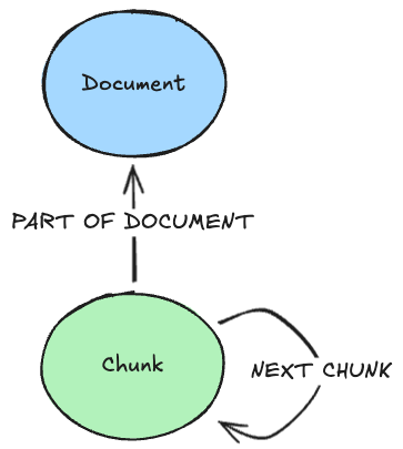
Core Lexical Data Model
The core lexical data model contains two nodes: Document and Chunk. These nodes are connected via a PART_OF_DOCUMENT relationship, and sequences of Chunk nodes are maintained by NEXT_CHUNK relationships. Document nodes can contain information such as the title, location URL, and authors. Chunk nodes may contain text, the text embedding, page numbers, and other metadata we’d like to use in filtering or citations.
In order to process a document, we must ensure that it’s in text format. Some documents, such as PDFs, must be converted to text via OCR or a similar method, such as VLM analysis. Once we have the document text and images parsed, it can then be partitioned. This involves breaking the document down into the smallest divisible text components. These include titles, lists, figure captions, and generic text, among other labels. The components are then aggregated according to our configuration to create the chunks we’ll ingest into our graph.

In Unstructured, we can use the partition_pdf function to partition and chunk a PDF document. We see a Python code example containing the configuration used below:
partitioned_doc = partition_pdf("articles/pdf/example.pdf",
strategy="hi_res",
extract_images_in_pdf=True,
extract_image_block_types=["Image", "Table"],
extract_image_block_to_payload=True,
chunking_strategy="by_title",
combine_text_under_n_chars=200,
max_characters=1000,
multipage_sections=True)
In the above example, we define many arguments to tune the PDF parsing. We set strategy="hi_res" and extract_images_in_pdf=True because we want to extract images from our document. Other strategy options include "fast" for text-only documents, "ocr_only" for extracting only the text from documents with text and images, and "vlm" for using a vision-language model to extract from complex, handwritten or multi-language content. We also want to extract the Base64 encoding of images and tables, so we must set extract_image_block_types=[“Image”, “Table”] and extract_image_block_to_payload=True. We set chunking_strategy="by_title", which will attempt to create the initial chunks by identifying sections broken up by Title components. We can also define the size of our final chunks with combine_text_under_n_chars=200 and max_characters=1000. The lower bound here is arbitrary, but the upper bound comes from Unstructured’s documentation, which states 1,000 characters to be the average paragraph length. Finally, we declare multipage_sections=True so we can combine content that spans across pages.
Images + Tables
Images and tables can be extracted from documents to supplement our retrieved context. Unstructured will parse these components into their own Unstructured Elements during partitioning, which can then be easily processed appropriately.

We can choose to store images and tables in an external store and create a pointer in Neo4j that allows us to retrieve the content during retrieval. Alternatively, we can generate Base64 encodings of image content and store the result as a node property in Neo4j. Then, upon retrieval, we can convert the Base64 string to an image and provide it alongside the text content in our LLM request. Tables can lso be extracted as markdown or HTML. If we extract a table in text format, we can store this text string in Neo4j as a node property as well.
When considering how to embed this content for similarity-based retrieval, we also have a few options. To perform similarity search over text and images in a shared embedding space, we can process using a multimodal embedding model, such as CLIP, to embed our text and images. We can also choose to generate text descriptions of images and tables, which may then be embedded. In this case, we only need to use a text embedding model for the embedding process. We can then store the resulting text description as a node property on the respective UnstructuredElement node or use the text to create a Chunk node. Either way allows us to return the description alongside the image for additional context.

Expanded Lexical Data Models
The core lexical data model serves as a starting point for your graph design. It may provide all the functionality you need for your use cases, but there are also instances where we may want to augment this data model.
We may want to change the core lexical data model to better reflect the structure of our documents. An easy way to start is by structuring our chunks by page. Typically, we’ll receive page numbers as a part of our processed chunk metadata. These are useful properties to store for citations, but we can also implement these as Page nodes in our graph. This better reflects the underlying document structure and simplifies some of our retrieval processes. With this model, we can easily reconstruct and retrieve full pages from our database. We also have the ability to match Chunk nodes and traverse to find the full page text for richer context.

Some other PDF parsers, such as PyMuPDF or docling, can automatically extract each page as an image, and each element with its respective bounding box coordinates on the page. This can be used to display the original document and highlight the source text, which is especially helpful for validating complex documents.
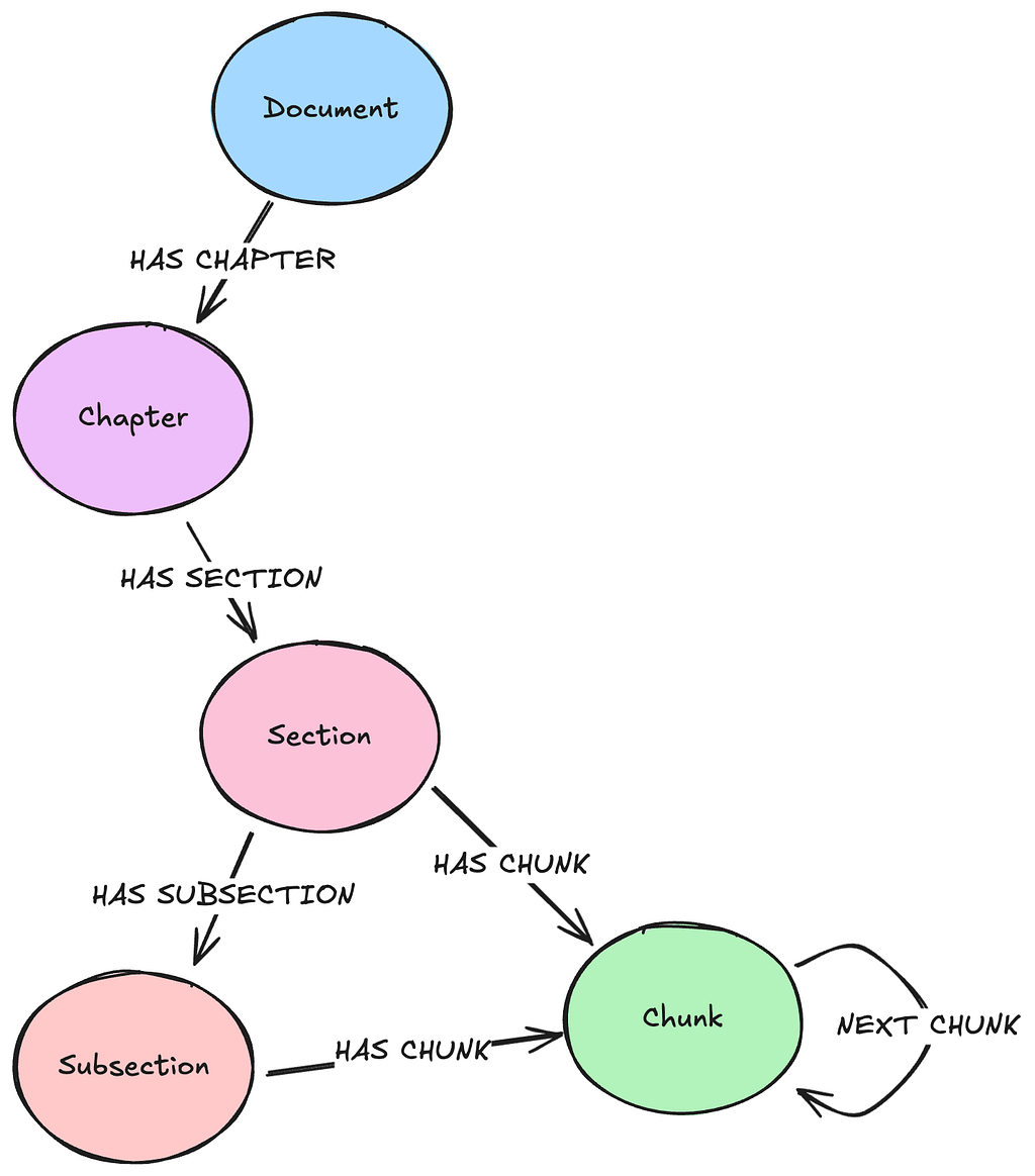
The page-based data model can be expanded upon by explicitly mapping out sections that exist within our document. This allows for more specific retrieval processes that can pull out only particular sections of a document at a time. This is useful if we’re generally interested in full sections, such as the methods or discussion sections of a research paper. In the example data model below, we see that both Section and Subsection nodes may have relationships with Chunk nodes. This is because some sections may not have subsections, so the Chunk nodes are derived from the full section content.
We can also augment our lexical data model in ways that aren’t related to the underlying document structure. A parent-child data model may offer improved retrieval results if we’re implementing vector similarity search in our application or have large text chunks. In this data model, we further divide our chunks (parents) into smaller chunks (children) and embed them instead of the parents. The smaller chunks here are not to be confused with the text elements discussed above during the partitioning process. During retrieval, we’ll perform a similarity search on the child Chunk nodes, then traverse to the parent Chunk nodes to gather the actual text content we want as context. Longer text may contain many diverse topics and have a resulting “noisy” embedding. By embedding smaller pieces of text, we’re creating more “pointed” embeddings that capture more specific meaning and should provide better matches for our similarity search. We still want to return the parent text since this contains both the child text and the surrounding context that supports our input query.

You can find more information on different lexical data models at GraphRAG.com.
Entity Extraction
The challenging aspect of knowledge graph generation is generating the entity subgraph of the domain component. This process is specific to the data domain and use cases of the graph. It’s also an iterative process with many configurable components and options. Here we’ll walk through some better practices of entity extraction that we hope will provide guidance as you develop your own pipelines.
Defining Entities
When we ask an LLM to extract entities, we’re providing a response model in the request that LLM may then map found entities to and return to us in JSON format. We can annotate these response models to provide context to the LLM as it decides which entities to extract. An effective way to do this is via the Pydantic Python library.
Pydantic allows us to explicitly define response models by creating them as Pydantic classes. We can also use the Pydantic Field object and field_validator function decorator that allows for advanced annotations and data massaging of each individual class property. This is a powerful tool that allows the model to throw explicit errors we can define within the validation functions when extracted content is incorrect. The LLM can then take these error messages and update the entity to adhere to our defined model. Pydantic models also allow us to define example JSON extracts within the class that will be passed when the model is exposed to the LLM. Here’s an example of how we can implement these concepts:
class Medication(BaseModel):
  """
  A substance used for medical treatment - a medicine or drug.
  This is a general representation of a medication.
  A Medication node may have relationships to TreatmentArm nodes that are specific to a particular study.
  """
  medication_class: str = Field(…, description="Drug class (e.g., GLP-1 RA, SGLT2i)")
  mechanism: Optional[str] = Field(None, description="Mechanism of action")
  generic_name: str = Field(…, description="Generic name of the medication")
  brand_names: Optional[List[str]] = Field(None, description="Commercial brand names")
  approval_status: Optional[str] = Field(None, description="FDA approval status")
  class Config:
  json_schema_extra = {
    "examples": [
      {
        "medication_class": "GLP-1 receptor agonist",
        "mechanism": "GLP-1 receptor activation",
        "generic_name": "semaglutide",
        "brand_names": ["ozempic", "wegovy", "rybelsus"],
        "approval_status": "FDA approved"
      }
    ]
  }

@field_validator("generic_name", "medication_class")
def validate_lower_case(cls, v: str) -> str:
  """
  Validate that the field value is all lower case.
  """
  return v.lower()

@field_validator("brand_names")
def validate_brand_names(cls, v: list[str] | None) -> list[str] | None:
  """
  Validate that the brand names are all lower case.
  """
  if v is not None:
    return [name.lower() for name in v]
  return v
Typically, we’ll pass many different entity options for the LLM to extract from a text chunk. When we do this, it’s crucial that we distinguish these entities not only via the class and field descriptions but also by how we name the class properties. For example, if we define both a Medication model and MedicalCondition model with only name and id fields, the LLM may return incorrect entities. This is because while the LLM will be aware that both these entities exist, it’ll only select the first model that matches that structure when it attempts to match its extracted JSON to a model. Since both these entities have the same JSON structure, only the first entity model seen by the LLM will be returned.

The solution here is to change the field names that we extract for each model. We can then map these extracted fields to the property names we would like during ingestion. So in the above example, Medication.medication_name may be ingested into Neo4j as Medication.name, and MedicalCondition.condition may be ingested as MedicalCondition.name.
Overstuffed Response Models
We’ll likely want to extract many entity types and their relationships from a text chunk. As we increase the number of entities and relationships in the response model, we’re also increasing the complexity of the extraction. This inherently increases the failure rate of extraction as the number of model options increases.
One method I found that helps address this is to provide the entity and relationship models in a nested Pydantic model. Originally, I started by providing only a list that contained a union of all entity and relationship models. This was unwieldy to process as the number of models increased and also began yielding poorer results. Providing a nested model as the response model instead is a more structured approach that is not only easier to parse in post-processing but also reduces the failure rate in my experience. Here, we provide a generic ResponseModel object that contains a field for each entity and relationship model. Each field’s value is then a list of the respective model. Our JSON response is now easier to understand and process:
class ResponseModel(BaseModel):
    """
    The response model for the extracted entities and relationships.
    """
    clinical_outcome: list[ClinicalOutcome] = Field(default_factory=list, description="The clinical outcomes in the chunk")
    treatment_arm: list[TreatmentArm] = Field(default_factory=list, description="The treatment arms in the chunk")
    study_population: list[StudyPopulation] = Field(default_factory=list, description="The study populations in the chunk")
    medical_condition: list[MedicalCondition] = Field(default_factory=list, description="The medical conditions in the chunk")
    medication: list[Medication] = Field(default_factory=list, description="The medications in the chunk")
    medication_used_in_treatment_arm: list[MedicationUsedInTreatmentArm] = Field(default_factory=list, description="The medications used in treatment arms in the chunk")
    treatment_arm_has_clinical_outcome: list[TreatmentArmHasClinicalOutcome] = Field(default_factory=list, description="The treatment arms that have clinical outcomes in the chunk")
    study_population_has_medical_condition: list[StudyPopulationHasMedicalCondition] = Field(default_factory=list, description="The study populations that have medical conditions in the chunk")
    study_population_in_treatment_arm: list[StudyPopulationInTreatmentArm] = Field(default_factory=list, description="The study populations that are in treatment arms in the chunk")
Another method is to identify subgraphs that exist in the entity graph and extract each subgraph in a separate call. This reduces the complexity of the response model, but at the cost of increasing the processing time and financial cost since we now need to process each chunk multiple times for each entity subgraph we identify. This method will hypothetically reduce our entity extraction failure rate and is a viable option for large entity schemas.

Context Management
The core context for entity extraction contains a few components. At a bare minimum, we should include the system message, instructions for extraction, the chunk text, and the response model. The system message will include general guidance on the role of the LLM and how it should behave. The following user message will contain the instructions and text to extract from. Our response model will be included alongside our messages in the API request. We use the Instructor library and OpenAI Chat Completions API to request a structured output response:
response = client.chat.completions.create(
            model="gpt-4o",
            messages=[
                {"role": "system", "content": system_prompt},
                {"role": "user", "content": user_prompt}
            ],
            response_model=ResponseModel,
            temperature=0.0
        )
This basic setup is usually fine for entity extraction, but there may be times when the current extraction process is dependent on knowledge of previously extracted entities. For example, we may be parsing processes and steps from an instructional document where processes contain a list of steps, and steps may contain child steps. Here, we must process the text chunks sequentially, and it’s imperative that we provide the previously extracted steps in the context so that the current extraction process maintains the current step sequence. Without it, we’ll lose the current position, and our final result will contain gaps. To address this, we can pass a list of the n most recent extracted steps in the context to inform the LLM where in the sequence it currently is.
The prompt below is used to present a rolling window of extracted steps in the context. We should extract entities serially so that we can provide the n most recent entities as our previous_processes variable.
Rules:
* Use the provided schema to extract Processes and Steps from the provided text.
* Follow the schema descriptions strictly.
* If there are existing Processes and Steps, you will have them as reference so you may append to them.
* If you are appending steps to an existing process you must use the existing process name and step ids.
* If a Step has no parent Step, then it must have a previous Step id noted! (only the very first Step in a process should not have a previous Step id)

Previous Processes and Steps:
{previous_processes}

Now extract Processes and Steps from the following text chunk:
{text_chunk}
Summary
Knowledge graph generation is a core component of how Neo4j fits into the GenAI ecosystem. It’s a powerful process that allows for novel insights and provides reliable and accurate context. The two core graph components — lexical and domain — each have their own considerations when developing the generation pipeline and may vary widely across different document types and data domains. This article details many of these considerations and provides examples to help guide your own knowledge graph development.
This field is relatively new and evolving quickly, so while these methods and strategies may change or become outdated in the future, they still provide a foundation for us to continue to iterate and improve upon.
Resources
- Amazon Textract
- Azure AI Document Intelligence
- Docling documentation
- Google Document AI
- GraphRAG concepts
- Hugging Face CLIP model documentation
- Instructor documentation
- LlamaParse documentation
- Neo4j Community Detection algorithm
- Neo4j-Field GitHub organization
- Neo4j Graph Data Science
- Neo4j Node Similarity algorithm
- OpenAI API Reference
- PubMed Knowledge Graph GitHub repo
- Pydantic documentation
- PyMuPDF documentation
- Unstructured documentation
- Vector Search Retriever
Knowledge Graph Generation was originally published in Neo4j Developer Blog on Medium, where people are continuing the conversation by highlighting and responding to this story.
The Developer’s Guide
Think knowledge graphs are too complex? They’re easier to build than you think. Learn step-by-step how to connect and organize your data with the relationships intact to query at speed.
Share Article


Explore
Related Articles

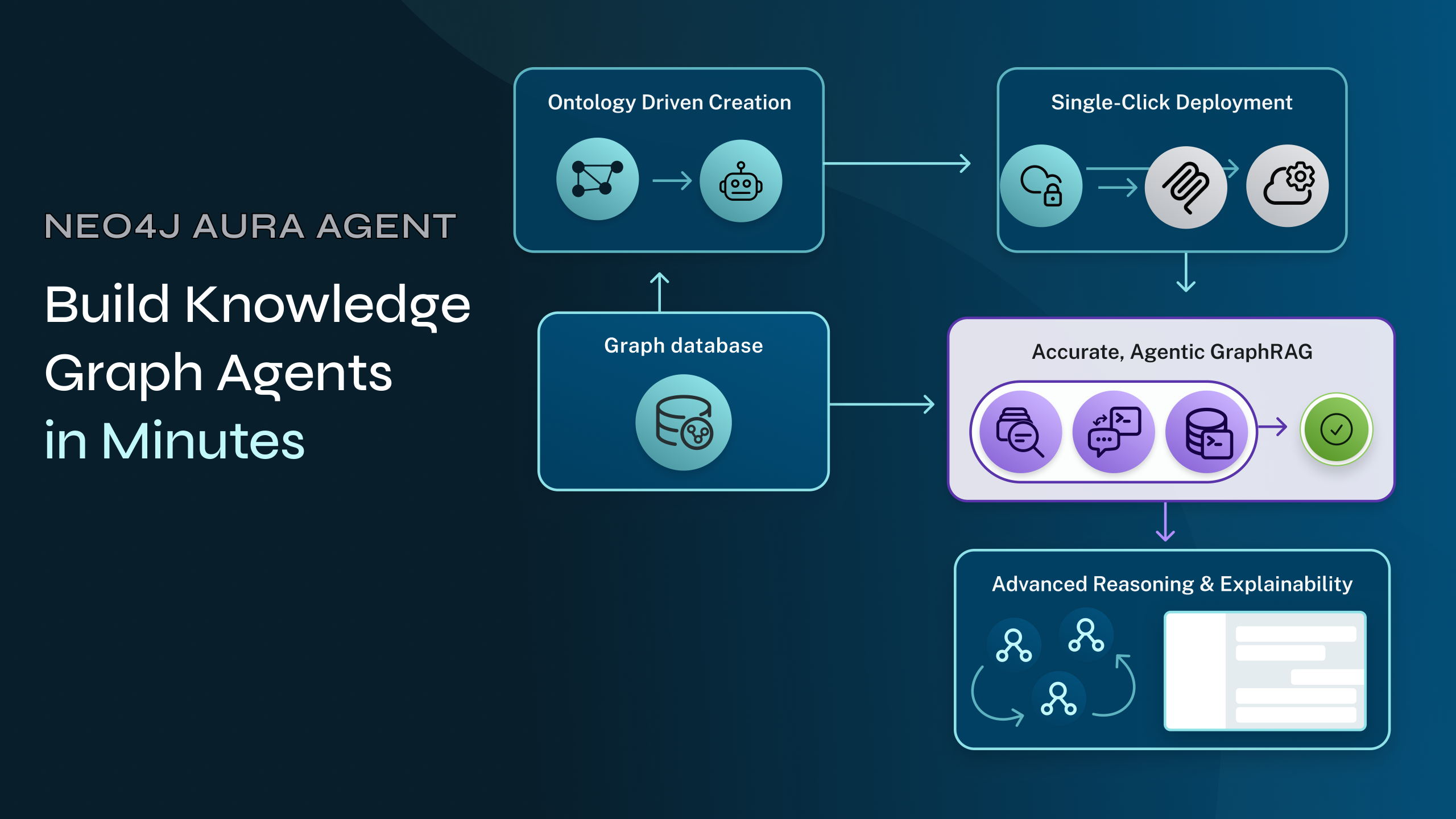
Graph-Driven AI for All: Neo4j Aura Agent Enters General Availability