Node Similarity

This section describes the Node Similarity algorithm in the Neo4j Graph Data Science library. The algorithm is based on the Jaccard and Overlap similarity metrics.

Directed

Undirected

Heterogeneous nodes

Heterogeneous relationships

Weighted relationships

Glossary

Directed: Directed trait. The algorithm is well-defined on a directed graph.
Directed: Directed trait. The algorithm ignores the direction of the graph.
Directed: Directed trait. The algorithm does not run on a directed graph.
Undirected: Undirected trait. The algorithm is well-defined on an undirected graph.
Undirected: Undirected trait. The algorithm ignores the undirectedness of the graph.
Heterogeneous nodes: Heterogeneous nodes fully supported. The algorithm has the ability to distinguish between nodes of different types.
Heterogeneous nodes: Heterogeneous nodes allowed. The algorithm treats all selected nodes similarly regardless of their label.
Heterogeneous relationships: Heterogeneous relationships fully supported. The algorithm has the ability to distinguish between relationships of different types.
Heterogeneous relationships: Heterogeneous relationships allowed. The algorithm treats all selected relationships similarly regardless of their type.
Weighted relationships: Weighted trait. The algorithm supports a relationship property to be used as weight, specified via the relationshipWeightProperty configuration parameter.
Weighted relationships: Weighted trait. The algorithm treats each relationship as equally important, discarding the value of any relationship weight.

Introduction

The Node Similarity algorithm compares a set of nodes based on the nodes they are connected to. Two nodes are considered similar if they share many of the same neighbors. Node Similarity computes pair-wise similarities based on the Jaccard metric, also known as the Jaccard Similarity Score, the Overlap coefficient, also known as the Szymkiewicz–Simpson coefficient, and the Cosine Similarity score. The first two are most frequently associated with unweighted sets, whereas Cosine with weighted input.

Given two sets A and B, the Jaccard Similarity is computed using the following formula:

The Overlap coefficient is computed using the following formula:

Formulas for the weighted case can be found in the weighted examples below.

The cosine similarity score is computed using the following formula, where entries are implicitly given a weight of 1 when A,B are unweighted:

The input of this algorithm is a bipartite, connected graph containing two disjoint node sets. Each relationship starts from a node in the first node set and ends at a node in the second node set.

The Node Similarity algorithm compares each node that has outgoing relationships with each other such node. For every node n, we collect the outgoing neighborhood N(n) of that node, that is, all nodes m such that there is a relationship from n to m. For each pair n, m, the algorithm computes a similarity for that pair that equals the outcome of the selected similarity metric for N(n) and N(m).

Node Similarity has time complexity O(n³) and space complexity O(n²). We compute and store neighbour sets in time and space O(n²), then compute pairwise similarity scores in time O(n³).

In order to bound memory usage you can specify an explicit limit on the number of results to output per node, this is the 'topK' parameter. It can be set to any value, except 0. You will lose precision in the overall computation of course, and running time is unaffected - we still have to compute results before potentially throwing them away.

The output of the algorithm are new relationships between pairs of the first node set. Similarity scores are expressed via relationship properties.

For more information on this algorithm, see:

It is also possible to apply filtering on the source and/or target nodes in the produced similarity pairs. You can consider the filtered Node Similarity algorithm for this purpose.

Running this algorithm requires sufficient available memory. Before running this algorithm, we recommend that you read Memory Estimation.

Syntax

This section covers the syntax used to execute the Node Similarity algorithm in each of its execution modes. We are describing the named graph variant of the syntax. To learn more about general syntax variants, see Syntax overview.

Node Similarity syntax per mode

Run Node Similarity in stream mode on a named graph.

CALL gds.nodeSimilarity.stream(
  graphName: String,
  configuration: Map
) YIELD
  node1: Integer,
  node2: Integer,
  similarity: Float

Table 1. Parameters
Name	Type	Default	Optional	Description
graphName	String	`n/a`	no	The name of a graph stored in the catalog.
configuration	Map	`{}`	yes	Configuration for algorithm-specifics and/or graph filtering.

Table 2. Configuration
Name	Type	Default	Optional	Description
nodeLabels	List of String	`['*']`	yes	Filter the named graph using the given node labels. Nodes with any of the given labels will be included.
relationshipTypes	List of String	`['*']`	yes	Filter the named graph using the given relationship types. Relationships with any of the given types will be included.
concurrency	Integer	`4`	yes	The number of concurrent threads used for running the algorithm.
jobId	String	`Generated internally`	yes	An ID that can be provided to more easily track the algorithm’s progress.
logProgress	Boolean	`true`	yes	If disabled the progress percentage will not be logged.
similarityCutoff	Float	`1E-42`	yes	Lower limit for the similarity score to be present in the result. Values must be between 0 and 1.
degreeCutoff	Integer	`1`	yes	Inclusive lower bound on the node degree for a node to be considered in the comparisons. This value can not be lower than 1.
upperDegreeCutoff	Integer	`2147483647`	yes	Inclusive upper bound on the node degree for a node to be considered in the comparisons. This value can not be lower than 1.
topK	Integer	`10`	yes	Limit on the number of scores per node. The K largest results are returned. This value cannot be lower than 1.
bottomK	Integer	`10`	yes	Limit on the number of scores per node. The K smallest results are returned. This value cannot be lower than 1.
topN	Integer	`0`	yes	Global limit on the number of scores computed. The N largest total results are returned. This value cannot be negative, a value of 0 means no global limit.
bottomN	Integer	`0`	yes	Global limit on the number of scores computed. The N smallest total results are returned. This value cannot be negative, a value of 0 means no global limit.
relationshipWeightProperty	String	`null`	yes	Name of the relationship property to use as weights. If unspecified, the algorithm runs unweighted.
similarityMetric	String	`JACCARD`	yes	The metric used to compute similarity. Can be either `JACCARD`, `OVERLAP` or `COSINE`.
useComponents	Boolean or String	`false`	yes	If enabled, Node Similarity will use components to improve the performance of the computation, skipping comparisons of nodes in different components. Set to `false` (Default): the algorithm does not use components, but computes similarity across the entire graph. Set to `true`: the algorithm uses components, and will compute these components before computing similarity. Set to String: use pre-computed components stored in the graph, with String as the key for a node property representing components

Table 3. Results
Name	Type	Description
`node1`	Integer	Node ID of the first node.
`node2`	Integer	Node ID of the second node.
`similarity`	Float	Similarity score for the two nodes.

Run Node Similarity in stats mode on a named graph.

CALL gds.nodeSimilarity.stats(
  graphName: String,
  configuration: Map
)
YIELD
  preProcessingMillis: Integer,
  computeMillis: Integer,
  postProcessingMillis: Integer,
  nodesCompared: Integer,
  similarityPairs: Integer,
  similarityDistribution: Map,
  configuration: Map

Table 4. Parameters
Name	Type	Default	Optional	Description
graphName	String	`n/a`	no	The name of a graph stored in the catalog.
configuration	Map	`{}`	yes	Configuration for algorithm-specifics and/or graph filtering.

Table 5. Configuration
Name	Type	Default	Optional	Description
nodeLabels	List of String	`['*']`	yes	Filter the named graph using the given node labels. Nodes with any of the given labels will be included.
relationshipTypes	List of String	`['*']`	yes	Filter the named graph using the given relationship types. Relationships with any of the given types will be included.
concurrency	Integer	`4`	yes	The number of concurrent threads used for running the algorithm.
jobId	String	`Generated internally`	yes	An ID that can be provided to more easily track the algorithm’s progress.
logProgress	Boolean	`true`	yes	If disabled the progress percentage will not be logged.
similarityCutoff	Float	`1E-42`	yes	Lower limit for the similarity score to be present in the result. Values must be between 0 and 1.
degreeCutoff	Integer	`1`	yes	Inclusive lower bound on the node degree for a node to be considered in the comparisons. This value can not be lower than 1.
upperDegreeCutoff	Integer	`2147483647`	yes	Inclusive upper bound on the node degree for a node to be considered in the comparisons. This value can not be lower than 1.
topK	Integer	`10`	yes	Limit on the number of scores per node. The K largest results are returned. This value cannot be lower than 1.
bottomK	Integer	`10`	yes	Limit on the number of scores per node. The K smallest results are returned. This value cannot be lower than 1.
topN	Integer	`0`	yes	Global limit on the number of scores computed. The N largest total results are returned. This value cannot be negative, a value of 0 means no global limit.
bottomN	Integer	`0`	yes	Global limit on the number of scores computed. The N smallest total results are returned. This value cannot be negative, a value of 0 means no global limit.
relationshipWeightProperty	String	`null`	yes	Name of the relationship property to use as weights. If unspecified, the algorithm runs unweighted.
similarityMetric	String	`JACCARD`	yes	The metric used to compute similarity. Can be either `JACCARD`, `OVERLAP` or `COSINE`.
useComponents	Boolean or String	`false`	yes	If enabled, Node Similarity will use components to improve the performance of the computation, skipping comparisons of nodes in different components. Set to `false` (Default): the algorithm does not use components, but computes similarity across the entire graph. Set to `true`: the algorithm uses components, and will compute these components before computing similarity. Set to String: use pre-computed components stored in the graph, with String as the key for a node property representing components

Table 6. Results
Name	Type	Description
preProcessingMillis	Integer	Milliseconds for preprocessing the data.
computeMillis	Integer	Milliseconds for running the algorithm.
postProcessingMillis	Integer	Milliseconds for computing component count and distribution statistics.
nodesCompared	Integer	The number of nodes for which similarity was computed.
similarityPairs	Integer	The number of similarities in the result.
similarityDistribution	Map	Map containing min, max, mean as well as p50, p75, p90, p95, p99 and p999 percentile values of the computed similarity results.
configuration	Map	The configuration used for running the algorithm.

Run Node Similarity in mutate mode on a graph stored in the catalog.

CALL gds.nodeSimilarity.mutate(
  graphName: String,
  configuration: Map
)
YIELD
  preProcessingMillis: Integer,
  computeMillis: Integer,
  mutateMillis: Integer,
  postProcessingMillis: Integer,
  relationshipsWritten: Integer,
  nodesCompared: Integer,
  similarityDistribution: Map,
  configuration: Map

Table 7. Parameters
Name	Type	Default	Optional	Description
graphName	String	`n/a`	no	The name of a graph stored in the catalog.
configuration	Map	`{}`	yes	Configuration for algorithm-specifics and/or graph filtering.

Table 8. Configuration
Name	Type	Default	Optional	Description
mutateRelationshipType	String	`n/a`	no	The relationship type used for the new relationships written to the projected graph.
mutateProperty	String	`n/a`	no	The relationship property in the GDS graph to which the similarity score is written.
nodeLabels	List of String	`['*']`	yes	Filter the named graph using the given node labels.
relationshipTypes	List of String	`['*']`	yes	Filter the named graph using the given relationship types.
concurrency	Integer	`4`	yes	The number of concurrent threads used for running the algorithm.
jobId	String	`Generated internally`	yes	An ID that can be provided to more easily track the algorithm’s progress.
similarityCutoff	Float	`1E-42`	yes	Lower limit for the similarity score to be present in the result. Values must be between 0 and 1.
degreeCutoff	Integer	`1`	yes	Inclusive lower bound on the node degree for a node to be considered in the comparisons. This value can not be lower than 1.
upperDegreeCutoff	Integer	`2147483647`	yes	Inclusive upper bound on the node degree for a node to be considered in the comparisons. This value can not be lower than 1.
topK	Integer	`10`	yes	Limit on the number of scores per node. The K largest results are returned. This value cannot be lower than 1.
bottomK	Integer	`10`	yes	Limit on the number of scores per node. The K smallest results are returned. This value cannot be lower than 1.
topN	Integer	`0`	yes	Global limit on the number of scores computed. The N largest total results are returned. This value cannot be negative, a value of 0 means no global limit.
bottomN	Integer	`0`	yes	Global limit on the number of scores computed. The N smallest total results are returned. This value cannot be negative, a value of 0 means no global limit.
relationshipWeightProperty	String	`null`	yes	Name of the relationship property to use as weights. If unspecified, the algorithm runs unweighted.
similarityMetric	String	`JACCARD`	yes	The metric used to compute similarity. Can be either `JACCARD`, `OVERLAP` or `COSINE`.
useComponents	Boolean or String	`false`	yes	If enabled, Node Similarity will use components to improve the performance of the computation, skipping comparisons of nodes in different components. Set to `false` (Default): the algorithm does not use components, but computes similarity across the entire graph. Set to `true`: the algorithm uses components, and will compute these components before computing similarity. Set to String: use pre-computed components stored in the graph, with String as the key for a node property representing components

Table 9. Results
Name	Type	Description
preProcessingMillis	Integer	Milliseconds for preprocessing the data.
computeMillis	Integer	Milliseconds for running the algorithm.
mutateMillis	Integer	Milliseconds for adding properties to the projected graph.
postProcessingMillis	Integer	Milliseconds for computing percentiles.
nodesCompared	Integer	The number of nodes for which similarity was computed.
relationshipsWritten	Integer	The number of relationships created.
similarityDistribution	Map	Map containing min, max, mean, stdDev and p1, p5, p10, p25, p75, p90, p95, p99, p100 percentile values of the computed similarity results.
configuration	Map	The configuration used for running the algorithm.

Run Node Similarity in write mode on a graph stored in the catalog.

CALL gds.nodeSimilarity.write(
  graphName: String,
  configuration: Map
)
YIELD
  preProcessingMillis: Integer,
  computeMillis: Integer,
  writeMillis: Integer,
  postProcessingMillis: Integer,
  nodesCompared: Integer,
  relationshipsWritten: Integer,
  similarityDistribution: Map,
  configuration: Map

Table 10. Parameters
Name	Type	Default	Optional	Description
graphName	String	`n/a`	no	The name of a graph stored in the catalog.
configuration	Map	`{}`	yes	Configuration for algorithm-specifics and/or graph filtering.

Table 11. Configuration
Name	Type	Default	Optional	Description
nodeLabels	List of String	`['*']`	yes	Filter the named graph using the given node labels. Nodes with any of the given labels will be included.
relationshipTypes	List of String	`['*']`	yes	Filter the named graph using the given relationship types. Relationships with any of the given types will be included.
concurrency	Integer	`4`	yes	The number of concurrent threads used for running the algorithm.
jobId	String	`Generated internally`	yes	An ID that can be provided to more easily track the algorithm’s progress.
logProgress	Boolean	`true`	yes	If disabled the progress percentage will not be logged.
writeConcurrency	Integer	`value of 'concurrency'`	yes	The number of concurrent threads used for writing the result to Neo4j.
writeRelationshipType	String	`n/a`	no	The relationship type used to persist the computed relationships in the Neo4j database.
writeProperty	String	`n/a`	no	The relationship property in the Neo4j database to which the similarity score is written.
similarityCutoff	Float	`1E-42`	yes	Lower limit for the similarity score to be present in the result. Values must be between 0 and 1.
degreeCutoff	Integer	`1`	yes	Inclusive lower bound on the node degree for a node to be considered in the comparisons. This value can not be lower than 1.
upperDegreeCutoff	Integer	`2147483647`	yes	Inclusive upper bound on the node degree for a node to be considered in the comparisons. This value can not be lower than 1.
topK	Integer	`10`	yes	Limit on the number of scores per node. The K largest results are returned. This value cannot be lower than 1.
bottomK	Integer	`10`	yes	Limit on the number of scores per node. The K smallest results are returned. This value cannot be lower than 1.
topN	Integer	`0`	yes	Global limit on the number of scores computed. The N largest total results are returned. This value cannot be negative, a value of 0 means no global limit.
bottomN	Integer	`0`	yes	Global limit on the number of scores computed. The N smallest total results are returned. This value cannot be negative, a value of 0 means no global limit.
relationshipWeightProperty	String	`null`	yes	Name of the relationship property to use as weights. If unspecified, the algorithm runs unweighted.
similarityMetric	String	`JACCARD`	yes	The metric used to compute similarity. Can be either `JACCARD`, `OVERLAP` or `COSINE`.
useComponents	Boolean or String	`false`	yes	If enabled, Node Similarity will use components to improve the performance of the computation, skipping comparisons of nodes in different components. Set to `false` (Default): the algorithm does not use components, but computes similarity across the entire graph. Set to `true`: the algorithm uses components, and will compute these components before computing similarity. Set to String: use pre-computed components stored in the graph, with String as the key for a node property representing components

Table 12. Results
Name	Type	Description
preProcessingMillis	Integer	Milliseconds for preprocessing data.
computeMillis	Integer	Milliseconds for running the algorithm.
writeMillis	Integer	Milliseconds for writing result data back to Neo4j.
postProcessingMillis	Integer	Milliseconds for computing percentiles.
nodesCompared	Integer	The number of nodes for which similarity was computed.
relationshipsWritten	Integer	The number of relationships created.
similarityDistribution	Map	Map containing min, max, mean, stdDev and p1, p5, p10, p25, p75, p90, p95, p99, p100 percentile values of the computed similarity results.
configuration	Map	The configuration used for running the algorithm.

Examples

All the examples below should be run in an empty database.

The examples use native projections as the norm, although Cypher projections can be used as well.

In this section we will show examples of running the Node Similarity algorithm on a concrete graph. The intention is to illustrate what the results look like and to provide a guide in how to make use of the algorithm in a real setting. We will do this on a small knowledge graph of a handful nodes connected in a particular pattern. The example graph looks like this:

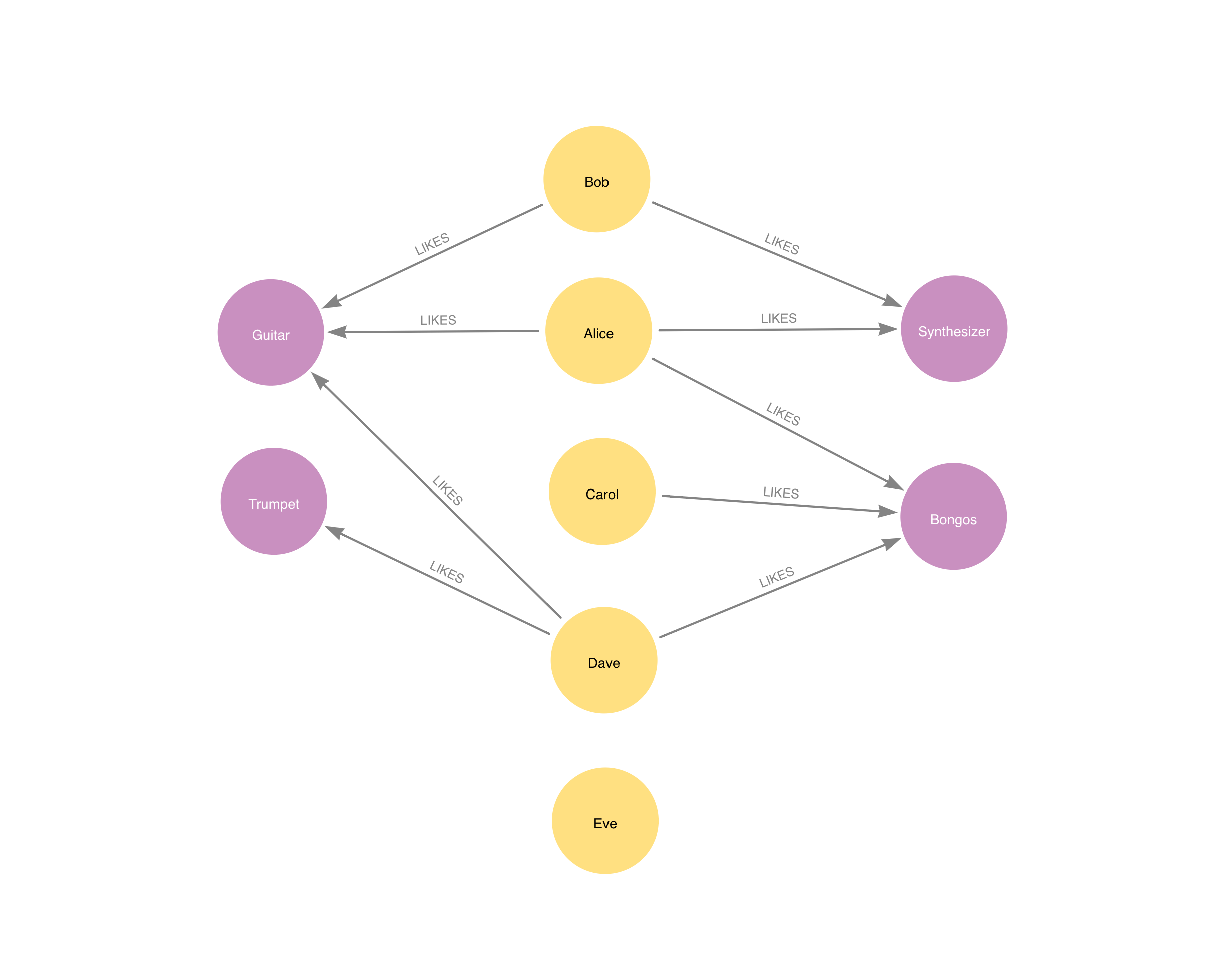
The following Cypher statement will create the example graph in the Neo4j database:

CREATE
  (alice:Person {name: 'Alice'}),
  (bob:Person {name: 'Bob'}),
  (carol:Person {name: 'Carol'}),
  (dave:Person {name: 'Dave'}),
  (eve:Person {name: 'Eve'}),
  (guitar:Instrument {name: 'Guitar'}),
  (synth:Instrument {name: 'Synthesizer'}),
  (bongos:Instrument {name: 'Bongos'}),
  (trumpet:Instrument {name: 'Trumpet'}),

  (alice)-[:LIKES]->(guitar),
  (alice)-[:LIKES]->(synth),
  (alice)-[:LIKES {strength: 0.5}]->(bongos),
  (bob)-[:LIKES]->(guitar),
  (bob)-[:LIKES]->(synth),
  (carol)-[:LIKES]->(bongos),
  (dave)-[:LIKES]->(guitar),
  (dave)-[:LIKES {strength: 1.5}]->(trumpet),
  (dave)-[:LIKES]->(bongos);

This bipartite graph has two node sets, Person nodes and Instrument nodes. The two node sets are connected via LIKES relationships. Each relationship starts at a Person node and ends at an Instrument node.

In the example, we want to use the Node Similarity algorithm to compare people based on the instruments they like.

The Node Similarity algorithm will only compute similarity for nodes that have a degree of at least 1. In the example graph, the Eve node will not be compared to other Person nodes.

The following statement will project the graph and store it in the graph catalog.

CALL gds.graph.project(
    'myGraph',
    ['Person', 'Instrument'],
    {
        LIKES: {
            properties: {
                strength: {
                    property: 'strength',
                    defaultValue: 1.0
                }
            }
        }
    }
);

In the following examples we will demonstrate using the Node Similarity algorithm on this graph.

Memory Estimation

First off, we will estimate the cost of running the algorithm using the estimate procedure. This can be done with any execution mode. We will use the write mode in this example. Estimating the algorithm is useful to understand the memory impact that running the algorithm on your graph will have. When you later actually run the algorithm in one of the execution modes the system will perform an estimation. If the estimation shows that there is a very high probability of the execution going over its memory limitations, the execution is prohibited. To read more about this, see Automatic estimation and execution blocking.

For more details on estimate in general, see Memory Estimation.

The following will estimate the memory requirements for running the algorithm:

CALL gds.nodeSimilarity.write.estimate('myGraph', {
  writeRelationshipType: 'SIMILAR',
  writeProperty: 'score'
})
YIELD nodeCount, relationshipCount, bytesMin, bytesMax, requiredMemory

Table 13. Results
nodeCount	relationshipCount	bytesMin	bytesMax	requiredMemory
9	9	2384	2600	"[2384 Bytes ... 2600 Bytes]"

Stream

In the stream execution mode, the algorithm returns the similarity score for each relationship. This allows us to inspect the results directly or post-process them in Cypher without any side effects.

For more details on the stream mode in general, see Stream.

The following will run the algorithm, and stream results:

CALL gds.nodeSimilarity.stream('myGraph')
YIELD node1, node2, similarity
RETURN gds.util.asNode(node1).name AS Person1, gds.util.asNode(node2).name AS Person2, similarity
ORDER BY similarity DESCENDING, Person1, Person2

Table 14. Results
Person1	Person2	similarity
"Alice"	"Bob"	0.6666666666666666
"Bob"	"Alice"	0.6666666666666666
"Alice"	"Dave"	0.5
"Dave"	"Alice"	0.5
"Alice"	"Carol"	0.3333333333333333
"Carol"	"Alice"	0.3333333333333333
"Carol"	"Dave"	0.3333333333333333
"Dave"	"Carol"	0.3333333333333333
"Bob"	"Dave"	0.25
"Dave"	"Bob"	0.25

We use default values for the procedure configuration parameter. TopK is set to 10, topN is set to 0. Because of that the result set contains the top 10 similarity scores for each node.

If we would like to instead compare the Instruments to each other, we would then project the LIKES relationship type using REVERSE orientation. This would return similarities for pairs of Instruments and not compute any similarities between Persons.

Stats

In the stats execution mode, the algorithm returns a single row containing a summary of the algorithm result. This execution mode does not have any side effects. It can be useful for evaluating algorithm performance by inspecting the computeMillis return item. In the examples below we will omit returning the timings. The full signature of the procedure can be found in the syntax section.

For more details on the stats mode in general, see Stats.

The following will run the algorithm and return the result in form of statistical and measurement values

CALL gds.nodeSimilarity.stats('myGraph')
YIELD nodesCompared, similarityPairs

Table 15. Results
nodesCompared	similarityPairs
4	10

Mutate

The mutate execution mode extends the stats mode with an important side effect: updating the named graph with a new relationship property containing the similarity score for that relationship. The name of the new property is specified using the mandatory configuration parameter mutateProperty. The result is a single summary row, similar to stats, but with some additional metrics. The mutate mode is especially useful when multiple algorithms are used in conjunction.

For more details on the mutate mode in general, see Mutate.

The following will run the algorithm, and write back results to the in-memory graph:

CALL gds.nodeSimilarity.mutate('myGraph', {
    mutateRelationshipType: 'SIMILAR',
    mutateProperty: 'score'
})
YIELD nodesCompared, relationshipsWritten

Table 16. Results
nodesCompared	relationshipsWritten
4	10

As we can see from the results, the number of created relationships is equal to the number of rows in the streaming example.

The relationships that are produced by the mutation are always directed, even if the input graph is undirected. If a → b is topK for a and symmetrically b → a is topK for b (or both a → b and b → a are topN), it appears as though an undirected relationship is produced. However, they are just two directed relationships that have been independently produced.

Write

The write execution mode for each pair of nodes creates a relationship with their similarity score as a property to the Neo4j database. The type of the new relationship is specified using the mandatory configuration parameter writeRelationshipType. The name of the new property is specified using the mandatory configuration parameter writeProperty. The result is a single summary row, similar to stats, but with some additional metrics.

For more details on the write mode in general, see Write.

The following will run the algorithm, and write back results:

CALL gds.nodeSimilarity.write('myGraph', {
    writeRelationshipType: 'SIMILAR',
    writeProperty: 'score'
})
YIELD nodesCompared, relationshipsWritten

Table 17. Results
nodesCompared	relationshipsWritten
4	10

As we can see from the results, the number of created relationships is equal to the number of rows in the streaming example.

The relationships that are written are always directed, even if the input graph is undirected. If a → b is topK for a and symmetrically b → a is topK for b (or both a → b and b → a are topN), it appears as though an undirected relationship is written. However, they are just two directed relationships that have been independently written.

Limit results

There are four limits that can be applied to the similarity results. Top limits the result to the highest similarity scores. Bottom limits the result to the lowest similarity scores. Both top and bottom limits can apply to the result as a whole ("N"), or to the result per node ("K").

There must always be a "K" limit, either bottomK or topK, which is a positive number. The default value for topK and bottomK is 10.

Table 18. Result limits
	total results	results per node
highest score	topN	topK
lowest score	bottomN	bottomK

topK and bottomK

TopK and bottomK are limits on the number of scores computed per node. For topK, the K largest similarity scores per node are returned. For bottomK, the K smallest similarity scores per node are returned. TopK and bottomK cannot be 0, used in conjunction, and the default value is 10. If neither is specified, topK is used.

The following will run the algorithm, and stream the top 1 result per node:

CALL gds.nodeSimilarity.stream('myGraph', { topK: 1 })
YIELD node1, node2, similarity
RETURN gds.util.asNode(node1).name AS Person1, gds.util.asNode(node2).name AS Person2, similarity
ORDER BY Person1

Table 19. Results
Person1	Person2	similarity
"Alice"	"Bob"	0.666666666666667
"Bob"	"Alice"	0.666666666666667
"Carol"	"Alice"	0.333333333333333
"Dave"	"Alice"	0.5

The following will run the algorithm, and stream the bottom 1 result per node:

CALL gds.nodeSimilarity.stream('myGraph', { bottomK: 1 })
YIELD node1, node2, similarity
RETURN gds.util.asNode(node1).name AS Person1, gds.util.asNode(node2).name AS Person2, similarity
ORDER BY Person1

Table 20. Results
Person1	Person2	similarity
"Alice"	"Carol"	0.3333333333333333
"Bob"	"Dave"	0.25
"Carol"	"Alice"	0.3333333333333333
"Dave"	"Bob"	0.25

topN and bottomN

TopN and bottomN limit the number of similarity scores across all nodes. This is a limit on the total result set, in addition to the topK or bottomK limit on the results per node. For topN, the N largest similarity scores are returned. For bottomN, the N smallest similarity scores are returned. A value of 0 means no global limit is imposed and all results from topK or bottomK are returned.

The following will run the algorithm, and stream the 3 highest out of the top 1 results per node:

CALL gds.nodeSimilarity.stream('myGraph', { topK: 1, topN: 3 })
YIELD node1, node2, similarity
RETURN gds.util.asNode(node1).name AS Person1, gds.util.asNode(node2).name AS Person2, similarity
ORDER BY similarity DESC, Person1, Person2

Table 21. Results
Person1	Person2	similarity
"Alice"	"Bob"	0.666666666666667
"Bob"	"Alice"	0.666666666666667
"Dave"	"Alice"	0.5

Degree cutoffs and similarity cutoff

Node Similarity can be tuned to ignore certain nodes based on degree constraints via two integer parameters named degreeCutoff and upperDegreeCutoff. If set, degreeCutoff imposes a lower limit on the degree in order for a node to be considered in the comparisons, and skips any nodes with degree below degreeCutoff. if set, upperDegreeCutoff imposes an upper limit on the node degree, and skips any nodes with degree higher than upperDegreeCutoff. The two parameters can also be combined so that only those nodes whose degree falls under a certain segment are considered.

The minimum value for both parameters is 1.

The following will ignore nodes with less than 3 LIKES relationships:

CALL gds.nodeSimilarity.stream('myGraph', { degreeCutoff: 3 })
YIELD node1, node2, similarity
RETURN gds.util.asNode(node1).name AS Person1, gds.util.asNode(node2).name AS Person2, similarity
ORDER BY Person1

Table 22. Results
Person1	Person2	similarity
"Alice"	"Dave"	0.5
"Dave"	"Alice"	0.5

Similarity cutoff is a lower limit for the similarity score to be present in the result. The default value is very small (1E-42) to exclude results with a similarity score of 0.

Setting similarity cutoff to 0 may yield a very large result set, increased runtime and memory consumption.

The following will ignore node pairs with a similarity score less than 0.5:

CALL gds.nodeSimilarity.stream('myGraph', { similarityCutoff: 0.5 })
YIELD node1, node2, similarity
RETURN gds.util.asNode(node1).name AS Person1, gds.util.asNode(node2).name AS Person2, similarity
ORDER BY Person1

Table 23. Results
Person1	Person2	similarity
"Alice"	"Bob"	0.666666666666667
"Alice"	"Dave"	0.5
"Bob"	"Alice"	0.6666666666666666
"Dave"	"Alice"	0.5

Weighted Similarity

Relationship properties can be used to modify the similarity induced by certain relationships by taking their value as a way of measuring importance. By default, Weighted node similarity uses weighted Jaccard similarity, according to the formula:

Formally, given two nodes and their weighted neighbour lists A' and B', we extend the lists to A and B, index over the union of their neighbours A' ∪ B' by setting weight = 0 for any non-neighbour, and then apply the weighted Jaccard similarity.

It also supports weighted Overlap similarity, according to the formula:

In addition, Cosine similarity can be used in the weighted case as mentioned in introduction.

Weighted similarity metrics are only defined for values greater or equal to 0.

The following query will respect relationship properties in the similarity computation:

CALL gds.nodeSimilarity.stream('myGraph', { relationshipWeightProperty: 'strength', similarityCutoff: 0.3 })
YIELD node1, node2, similarity
RETURN gds.util.asNode(node1).name AS Person1, gds.util.asNode(node2).name AS Person2, similarity
ORDER BY Person1

Table 24. Results
Person1	Person2	similarity
"Alice"	"Bob"	0.8
"Alice"	"Dave"	0.333333333333333
"Bob"	"Alice"	0.8
"Dave"	"Alice"	0.333333333333333

It can be seen that the similarity between Alice and Dave decreased (from 0.5 to 0.33) compared to the non-weighted version of this algorithm.

Alice likes Guitar, Synthesize and Bongos with strengths (1, 1, 0.5). Dave likes Guitar, Bongos and Trumpet with strengths (1, 1, 1.5). Therefore, taking Alice and Dave’s neighbours, we have list of strengths for Alice as A = (1, 1, 0.5, 0) and for Dave B = (1, 0, 1, 1.5), indexed as Guitar, Synthesizer, Bongos, Trumpet.

The weighted (Jaccard) node similarity of Alice and Dave is hence:

Analogously, the similarity between Alice and Bob increased (from 0.66 to 0.8) as the missing liked instrument has a lower impact on the similarity score.