Graph Data Science integration
Neo4j Graph Data Science algorithms can help you find new insights in your data, both into the nodes themselves as well as into how they are connected. See The Neo4j Graph Data Science Library Manual for more information on graph algorithms.
|
Running Graph Data Science algorithms on elements in your Scene does not alter the underlying data. The scores only exist temporarily in Bloom. However, if you opt to create a projection on the entire graph, results are written back to your data as a new database property. |
The algorithms are described briefly below, but please refer to The Neo4j Graph Data Science Library Manual for their full descriptions.
|
In order to use GDS functionality in Bloom, you need to have a supported version of the GDS plugin installed. See Version compatibility and Neo4j Graph Data Science Library Manual → Supported Neo4j versions for more information. |
Available GDS algorithms in Bloom
The available algorithms can be divided into two categories, centrality and community detection. Centrality algorithms are used to measure the importance of particular nodes in a network and to discover the roles individual nodes play. A node’s importance can mean that it has a lot of connections or that it is transitively connected to other important nodes. It can also mean that another node can be reached in few hops or that it sits on the shortest path of multiple pairs of nodes. The following centrality algorithms are available in Bloom:
-
Betweenness Centrality
-
Degree Centrality
-
Eigenvector Centrality
-
PageRank
Community detection algorithms on the other hand, are used to find sub-groups within the data and can give insight to whether networks are likely to break apart. Community detection is useful in a variety of graphs, from social media networks to machine learning. The following community detection algorithms are available in Bloom:
-
Louvain
-
Label propagation
-
Weakly connected components
Degree Centrality
The Degree Centrality algorithm measures the relationships connected to a node, either incoming, outgoing, or both, to find the most connected nodes in a graph.
Betweenness Centrality
The Betweenness Centrality algorithm finds influential nodes, that is, nodes that are thoroughfares for the most shortest-paths in the scene. Nodes with a high degree of betweenness centrality are nodes that connect different sub-parts of a graph.
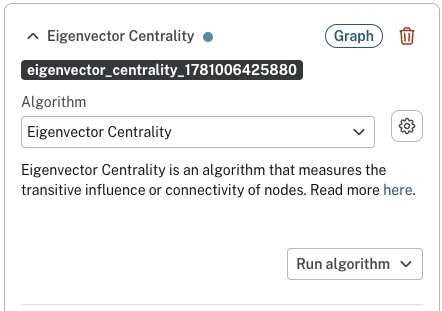
Eigenvector Centrality
The Eigenvector Centrality algorithm is used to measure transitive influence of nodes. That means that for a node to score a high eigenvector centrality, it needs to be connected to other nodes which in turn are well-connected. The difference between the eigenvector and the betweenness centrality is that the eigenvector is not only based on a node’s direct relationships with other nodes, but on the relationships of the related nodes as well.
PageRank
The PageRank alggorithm is a way to measure the relevance of each node in a graph. The relevance of a node is based on how many incoming relationships from other nodes it has and how important the source nodes are.
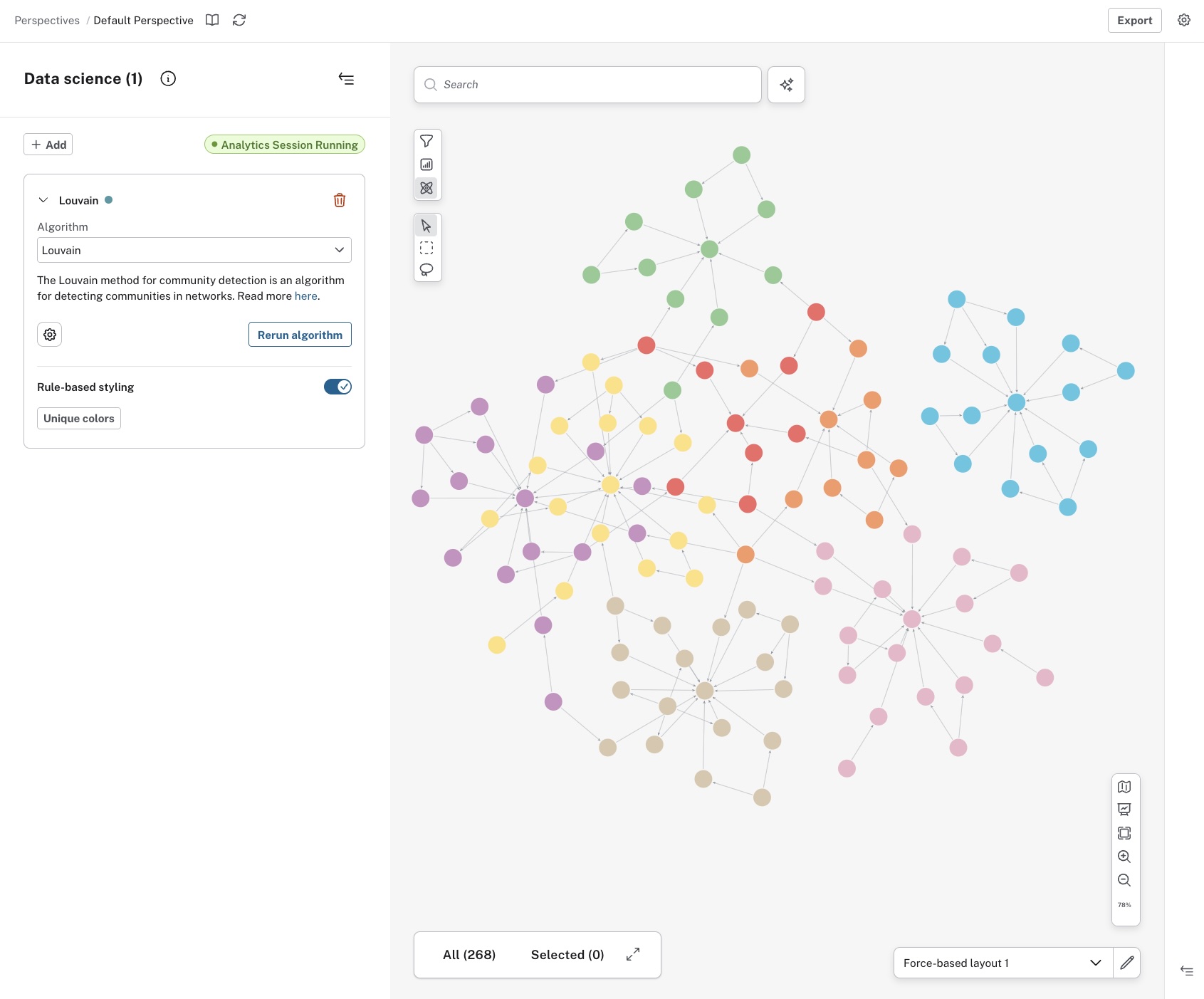
Louvain
The Louvain algorithm aims to find clusters of highly connected nodes within a larger network. It can be useful for product recommendations, for example. If you know a customer bought one product from an identified cluster, they are likely to be interested in another product from that cluster.
Label Propagation
The Label Propagation algorithm is another way to find communities in a graph. One difference between Label Propagation and Louvain, both community detection algorithms, is that this one allows for some supervision, i.e. it is possible to set certain prerequisites that allows for a degree of control of the outcome. This can be useful when you already have some knowledge of the intrinsic structure of your data.
Weakly Connected Components
The Weakly Connected Components algorithm finds subgraphs that are unreachable from other parts of the graph. It can be used to determine whether your network is fully connected or not and also to find vulnerable parts in supply chains, for example.
Using GDS algorithms in Bloom
Prerequisites
To use GDS algorithms in Bloom, there are two things you need to do before you start Bloom:
-
Install the Graph Data Science Library plugin. The easiest way to do this is in Neo4j Desktop. See the Install a plugin section in the Neo4j Desktop manual for more information.
-
Allow GDS in the
neo4j.conffile. This can be done manually or via Neo4j Desktop. Thedbms.security.procedures.unrestrictedsetting needs to include both Bloom and GDS (and others that are already specified) as such:dbms.security.procedures.unrestricted=jwt.security.*,bloom.*,gds.*,apoc.*The
dbms.security.procedures.allowlistsetting needs to be uncommented and also needs to include both Bloom and GDS (and others, as mentioned previously) as such:dbms.security.procedures.allowlist=apoc.coll.*,apoc.load.*,gds.*,bloom.*,apoc.*
With these in place, you can start Bloom and start searching to bring some data to your Scene to run the algorithms on.
Alternatively, if you connect to a Neo4j Aura instance, GDS algorithms can run either in a separate compute environment via the serverless option, or in the same AuraDB instance as the database using the Graph Analytics plugin, sharing resources. This is selected when you create an AuraDB instance in the Neo4j Aura console. For more information, see Neo4j Aura → Create an instance.
Running the algorithms
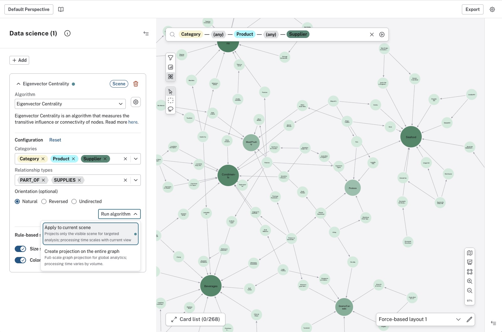
The GDS algorithms are accessed via the GDS button in the upper-left corner of the Scene. When you have selected an appropriate algorithm, you have the option to run it on all elements in the Scene, or specify which node categories and/or relationship types. Additionally, you can also select the orientation of the relationships to be traversed. The options are accessed via the Settings button in the GDS drawer.
When you are satisfied, you can either run the algorithm on the data in your current Scene or create a projection on the entire graph. The time it takes to run the algorithm can be different depending on the size of your graph. Additionally, running an algorithm on the current Scene only temporarily adds a score to the elements in the Scene. This action does not write to your graph. But creating a projection on the entire graph adds a new database property containing the individual score to all affected elements. The property name contains the name of the algorithm and a number and it is displayed in the GDS drawer.
You can edit and delete the property on the individual nodes, but you cannot rename it. You can manually remove the property from the entire graph using a Cypher query in Neo4j Browser, for example, if needed.
Applying your selected algorithm does not immediately change anything in the Scene. You can inspect each node to see its score, but to make the results easily visible, apply rule-based styling. This is done directly in the GDS drawer. The centrality algorithms are based on a range of values and can be either size-scaled or color gradient, while the community detection algorithms use unique values and offer unique colors to style the nodes.