Betweenness Centrality
Glossary
- Directed
-
Directed trait. The algorithm is well-defined on a directed graph.
- Directed
-
Directed trait. The algorithm ignores the direction of the graph.
- Directed
-
Directed trait. The algorithm does not run on a directed graph.
- Undirected
-
Undirected trait. The algorithm is well-defined on an undirected graph.
- Undirected
-
Undirected trait. The algorithm ignores the undirectedness of the graph.
- Heterogeneous nodes
-
Heterogeneous nodes fully supported. The algorithm has the ability to distinguish between nodes of different types.
- Heterogeneous nodes
-
Heterogeneous nodes allowed. The algorithm treats all selected nodes similarly regardless of their label.
- Heterogeneous relationships
-
Heterogeneous relationships fully supported. The algorithm has the ability to distinguish between relationships of different types.
- Heterogeneous relationships
-
Heterogeneous relationships allowed. The algorithm treats all selected relationships similarly regardless of their type.
- Weighted relationships
-
Weighted trait. The algorithm supports a relationship property to be used as weight, specified via the relationshipWeightProperty configuration parameter.
- Weighted relationships
-
Weighted trait. The algorithm treats each relationship as equally important, discarding the value of any relationship weight.
- Node properties
-
Node properties trait. The algorithm makes use of node properties.
Introduction
Betweenness centrality is a way of detecting the amount of influence a node has over the flow of information in a graph. It is often used to find nodes that serve as a bridge from one part of a graph to another.
The algorithm calculates shortest paths between all pairs of nodes in a graph. Each node receives a score, based on the number of shortest paths that pass through the node. Nodes that more frequently lie on shortest paths between other nodes will have higher betweenness centrality scores.
Betweenness centrality is implemented for graphs without weights or with positive weights. The GDS implementation is based on Brandes' approximate algorithm for unweighted graphs. For weighted graphs, multiple concurrent Dijkstra algorithms are used. The implementation requires O(n + m) space and runs in O(n * m) time, where n is the number of nodes and m the number of relationships in the graph.
For more information on this algorithm, see:
|
Running this algorithm requires sufficient memory availability. Before running this algorithm, we recommend that you read Memory Estimation. |
Considerations and sampling
The Betweenness Centrality algorithm can be very resource-intensive to compute. Brandes' approximate algorithm computes single-source shortest paths (SSSP) for a set of source nodes. When all nodes are selected as source nodes, the algorithm produces an exact result. However, for large graphs this can potentially lead to very long runtimes. Thus, approximating the results by computing the SSSPs for only a subset of nodes can be useful. In GDS we refer to this technique as sampling, where the size of the source node set is the sampling size.
There are two things to consider when executing the algorithm on large graphs:
-
A higher parallelism leads to higher memory consumption as each thread executes SSSPs for a subset of source nodes sequentially.
-
In the worst case, a single SSSP requires the whole graph to be duplicated in memory.
-
-
A higher sampling size leads to more accurate results, but also to a potentially much longer execution time.
Changing the values of the configuration parameters concurrency and samplingSize, respectively, can help to manage these considerations.
Sampling strategies
Brandes defines several strategies for selecting source nodes. The GDS implementation is based on the random degree selection strategy, which selects nodes with a probability proportional to their degree. The idea behind this strategy is that such nodes are likely to lie on many shortest paths in the graph and thus have a higher contribution to the betweenness centrality score.
Syntax
This section covers the syntax used to execute the Betweenness Centrality algorithm in each of its execution modes. We are describing the named graph variant of the syntax. To learn more about general syntax variants, see Syntax overview.
CALL gds.betweenness.stream(
  graphName: String,
  configuration: Map
)
YIELD
  nodeId: Integer,
score: Float| Name | Type | Default | Optional | Description |
|---|---|---|---|---|
graphName |
String |
|
no |
The name of a graph stored in the catalog. |
configuration |
Map |
|
yes |
Configuration for algorithm-specifics and/or graph filtering. |
| Name | Type | Default | Optional | Description |
|---|---|---|---|---|
List of String |
|
yes |
Filter the named graph using the given node labels. Nodes with any of the given labels will be included. |
|
List of String |
|
yes |
Filter the named graph using the given relationship types. Relationships with any of the given types will be included. |
|
Integer |
|
yes |
The number of concurrent threads used for running the algorithm. |
|
String |
|
yes |
An ID that can be provided to more easily track the algorithm’s progress. |
|
Boolean |
|
yes |
If disabled the progress percentage will not be logged. |
|
samplingSize |
Integer |
|
yes |
The number of source nodes to consider for computing centrality scores. |
samplingSeed |
Integer |
|
yes |
The seed value for the random number generator that selects start nodes. |
String |
|
yes |
Name of the relationship property to use as weights. If unspecified, the algorithm runs unweighted. |
|
1. In a GDS Session, the default is the number of available processors. |
||||
| Name | Type | Description |
|---|---|---|
nodeId |
Integer |
Node ID. |
score |
Float |
Betweenness Centrality score. |
CALL gds.betweenness.stats(
  graphName: String,
  configuration: Map
)
YIELD
  centralityDistribution: Map,
  preProcessingMillis: Integer,
  computeMillis: Integer,
  postProcessingMillis: Integer,
configuration: Map| Name | Type | Default | Optional | Description |
|---|---|---|---|---|
graphName |
String |
|
no |
The name of a graph stored in the catalog. |
configuration |
Map |
|
yes |
Configuration for algorithm-specifics and/or graph filtering. |
| Name | Type | Default | Optional | Description |
|---|---|---|---|---|
List of String |
|
yes |
Filter the named graph using the given node labels. Nodes with any of the given labels will be included. |
|
List of String |
|
yes |
Filter the named graph using the given relationship types. Relationships with any of the given types will be included. |
|
Integer |
|
yes |
The number of concurrent threads used for running the algorithm. |
|
String |
|
yes |
An ID that can be provided to more easily track the algorithm’s progress. |
|
Boolean |
|
yes |
If disabled the progress percentage will not be logged. |
|
samplingSize |
Integer |
|
yes |
The number of source nodes to consider for computing centrality scores. |
samplingSeed |
Integer |
|
yes |
The seed value for the random number generator that selects start nodes. |
String |
|
yes |
Name of the relationship property to use as weights. If unspecified, the algorithm runs unweighted. |
|
2. In a GDS Session, the default is the number of available processors. |
||||
| Name | Type | Description |
|---|---|---|
centralityDistribution |
Map |
Map containing min, max, mean as well as p50, p75, p90, p95, p99 and p999 percentile values of centrality values. |
preProcessingMillis |
Integer |
Milliseconds for preprocessing the graph. |
computeMillis |
Integer |
Milliseconds for running the algorithm. |
postProcessingMillis |
Integer |
Milliseconds for computing the statistics. |
configuration |
Map |
Configuration used for running the algorithm. |
CALL gds.betweenness.mutate(
  graphName: String,
  configuration: Map
)
YIELD
  centralityDistribution: Map,
  preProcessingMillis: Integer,
  computeMillis: Integer,
  postProcessingMillis: Integer,
  mutateMillis: Integer,
  nodePropertiesWritten: Integer,
configuration: Map| Name | Type | Default | Optional | Description |
|---|---|---|---|---|
graphName |
String |
|
no |
The name of a graph stored in the catalog. |
configuration |
Map |
|
yes |
Configuration for algorithm-specifics and/or graph filtering. |
| Name | Type | Default | Optional | Description |
|---|---|---|---|---|
mutateProperty |
String |
|
no |
The node property in the GDS graph to which the centrality is written. |
List of String |
|
yes |
Filter the named graph using the given node labels. |
|
List of String |
|
yes |
Filter the named graph using the given relationship types. |
|
Integer |
|
yes |
The number of concurrent threads used for running the algorithm. |
|
Boolean |
|
yes |
If disabled the progress percentage will not be logged. |
|
String |
|
yes |
An ID that can be provided to more easily track the algorithm’s progress. |
|
samplingSize |
Integer |
|
yes |
The number of source nodes to consider for computing centrality scores. |
samplingSeed |
Integer |
|
yes |
The seed value for the random number generator that selects start nodes. |
String |
|
yes |
Name of the relationship property to use as weights. If unspecified, the algorithm runs unweighted. |
| Name | Type | Description |
|---|---|---|
centralityDistribution |
Map |
Map containing min, max, mean as well as p50, p75, p90, p95, p99 and p999 percentile values of centrality values. |
preProcessingMillis |
Integer |
Milliseconds for preprocessing the graph. |
computeMillis |
Integer |
Milliseconds for running the algorithm. |
postProcessingMillis |
Integer |
Milliseconds for computing the statistics. |
mutateMillis |
Integer |
Milliseconds for adding properties to the in-memory graph. |
nodePropertiesWritten |
Integer |
Number of properties added to the in-memory graph. |
configuration |
Map |
Configuration used for running the algorithm. |
CALL gds.betweenness.write(
  graphName: String,
  configuration: Map
)
YIELD
  centralityDistribution: Map,
  preProcessingMillis: Integer,
  computeMillis: Integer,
  postProcessingMillis: Integer,
  writeMillis: Integer,
  nodePropertiesWritten: Integer,
configuration: Map| Name | Type | Default | Optional | Description |
|---|---|---|---|---|
graphName |
String |
|
no |
The name of a graph stored in the catalog. |
configuration |
Map |
|
yes |
Configuration for algorithm-specifics and/or graph filtering. |
| Name | Type | Default | Optional | Description |
|---|---|---|---|---|
List of String |
|
yes |
Filter the named graph using the given node labels. Nodes with any of the given labels will be included. |
|
List of String |
|
yes |
Filter the named graph using the given relationship types. Relationships with any of the given types will be included. |
|
Integer |
|
yes |
The number of concurrent threads used for running the algorithm. |
|
String |
|
yes |
An ID that can be provided to more easily track the algorithm’s progress. |
|
Boolean |
|
yes |
If disabled the progress percentage will not be logged. |
|
Integer |
|
yes |
The number of concurrent threads used for writing the result to Neo4j. |
|
String |
|
no |
The node property in the Neo4j database to which the centrality is written. |
|
samplingSize |
Integer |
|
yes |
The number of source nodes to consider for computing centrality scores. |
samplingSeed |
Integer |
|
yes |
The seed value for the random number generator that selects start nodes. |
String |
|
yes |
Name of the relationship property to use as weights. If unspecified, the algorithm runs unweighted. |
|
3. In a GDS Session, the default is the number of available processors. |
||||
| Name | Type | Description |
|---|---|---|
centralityDistribution |
Map |
Map containing min, max, mean as well as p50, p75, p90, p95, p99 and p999 percentile values of centrality values. |
preProcessingMillis |
Integer |
Milliseconds for preprocessing the graph. |
computeMillis |
Integer |
Milliseconds for running the algorithm. |
postProcessingMillis |
Integer |
Milliseconds for computing the statistics. |
writeMillis |
Integer |
Milliseconds for writing result data back. |
nodePropertiesWritten |
Integer |
Number of properties written to Neo4j. |
configuration |
Map |
The configuration used for running the algorithm. |
Examples
|
All the examples below should be run in an empty database. The examples use Cypher projections as the norm. Native projections will be deprecated in a future release. |
In this section we will show examples of running the Betweenness Centrality algorithm on a concrete graph. The intention is to illustrate what the results look like and to provide a guide in how to make use of the algorithm in a real setting. We will do this on a small social network graph of a handful nodes connected in a particular pattern. The example graph looks like this:
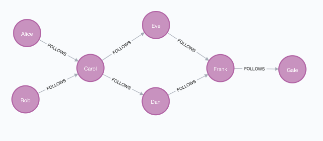
CREATE
  (alice:User {name: 'Alice'}),
  (bob:User {name: 'Bob'}),
  (carol:User {name: 'Carol'}),
  (dan:User {name: 'Dan'}),
  (eve:User {name: 'Eve'}),
  (frank:User {name: 'Frank'}),
  (gale:User {name: 'Gale'}),

  (alice)-[:FOLLOWS {weight: 1.0}]->(carol),
  (bob)-[:FOLLOWS {weight: 1.0}]->(carol),
  (carol)-[:FOLLOWS {weight: 1.0}]->(dan),
  (carol)-[:FOLLOWS {weight: 1.3}]->(eve),
  (dan)-[:FOLLOWS {weight: 1.0}]->(frank),
  (eve)-[:FOLLOWS {weight: 0.5}]->(frank),
  (frank)-[:FOLLOWS {weight: 1.0}]->(gale);
With the graph in Neo4j we can now project it into the graph catalog to prepare it for algorithm execution.
We do this using a Cypher projection targeting the User nodes and the FOLLOWS relationships.
MATCH (source:User)-[r:FOLLOWS]->(target:User)
RETURN gds.graph.project(
  'myGraph',
  source,
  target,
  { relationshipProperties: r { .weight } }
)
In the following examples we will demonstrate using the Betweenness Centrality algorithm on this graph.
Memory Estimation
First off, we will estimate the cost of running the algorithm using the estimate procedure.
This can be done with any execution mode.
We will use the write mode in this example.
Estimating the algorithm is useful to understand the memory impact that running the algorithm on your graph will have.
When you later actually run the algorithm in one of the execution modes the system will perform an estimation.
If the estimation shows that there is a very high probability of the execution going over its memory limitations, the execution is prohibited.
To read more about this, see Automatic estimation and execution blocking.
For more details on estimate in general, see Memory Estimation.
CALL gds.betweenness.write.estimate('myGraph', { writeProperty: 'betweenness' })
YIELD nodeCount, relationshipCount, bytesMin, bytesMax, requiredMemory| nodeCount | relationshipCount | bytesMin | bytesMax | requiredMemory |
|---|---|---|---|---|
7 |
7 |
2944 |
2944 |
"2944 Bytes" |
As is discussed in Considerations and sampling we can configure the memory requirements using the concurrency configuration parameter.
CALL gds.betweenness.write.estimate('myGraph', { writeProperty: 'betweenness', concurrency: 1 })
YIELD nodeCount, relationshipCount, bytesMin, bytesMax, requiredMemory| nodeCount | relationshipCount | bytesMin | bytesMax | requiredMemory |
|---|---|---|---|---|
7 |
7 |
856 |
856 |
"856 Bytes" |
Here we can note that the estimated memory requirements were lower than when running with the default concurrency setting. Similarly, using a higher value will increase the estimated memory requirements.
Stream
In the stream execution mode, the algorithm returns the centrality for each node.
This allows us to inspect the results directly or post-process them in Cypher without any side effects.
For example, we can order the results to find the nodes with the highest betweenness centrality.
For more details on the stream mode in general, see Stream.
stream mode:CALL gds.betweenness.stream('myGraph')
YIELD nodeId, score
RETURN gds.util.asNode(nodeId).name AS name, score
ORDER BY name ASC| name | score |
|---|---|
"Alice" |
0.0 |
"Bob" |
0.0 |
"Carol" |
8.0 |
"Dan" |
3.0 |
"Eve" |
3.0 |
"Frank" |
5.0 |
"Gale" |
0.0 |
We note that the 'Carol' node has the highest score, followed by the 'Frank' node. Studying the example graph we can see that these nodes are in bottleneck positions in the graph. The 'Carol' node connects the 'Alice' and 'Bob' nodes to all other nodes, which increases its score. In particular, the shortest path from 'Alice' or 'Bob' to any other reachable node passes through 'Carol'. Similarly, all shortest paths that lead to the 'Gale' node passes through the 'Frank' node. Since 'Gale' is reachable from each other node, this causes the score for 'Frank' to be high.
Conversely, there are no shortest paths that pass through either of the nodes 'Alice', 'Bob' or 'Gale' which causes their betweenness centrality score to be zero.
Stats
In the stats execution mode, the algorithm returns a single row containing a summary of the algorithm result.
In particular, Betweenness Centrality returns the minimum, maximum and sum of all centrality scores.
This execution mode does not have any side effects.
It can be useful for evaluating algorithm performance by inspecting the computeMillis return item.
In the examples below we will omit returning the timings.
The full signature of the procedure can be found in the syntax section.
For more details on the stats mode in general, see Stats.
stats mode:CALL gds.betweenness.stats('myGraph')
YIELD centralityDistribution
RETURN centralityDistribution.min AS minimumScore, centralityDistribution.mean AS meanScore| minimumScore | meanScore |
|---|---|
0.0 |
2.714292253766741 |
Comparing this to the results we saw in the stream example, we can find our minimum and maximum values from the table. It is worth noting that unless the graph has a particular shape involving a directed cycle, the minimum score will almost always be zero.
Mutate
The mutate execution mode extends the stats mode with an important side effect: updating the named graph with a new node property containing the centrality for that node.
The name of the new property is specified using the mandatory configuration parameter mutateProperty.
The result is a single summary row, similar to stats, but with some additional metrics.
The mutate mode is especially useful when multiple algorithms are used in conjunction.
For more details on the mutate mode in general, see Mutate.
mutate mode:CALL gds.betweenness.mutate('myGraph', { mutateProperty: 'betweenness' })
YIELD centralityDistribution, nodePropertiesWritten
RETURN centralityDistribution.min AS minimumScore, centralityDistribution.mean AS meanScore, nodePropertiesWritten| minimumScore | meanScore | nodePropertiesWritten |
|---|---|---|
0.0 |
2.7142922538 |
7 |
The returned result is the same as in the stats example.
Additionally, the graph 'myGraph' now has a node property betweenness which stores the betweenness centrality score for each node.
To find out how to inspect the new schema of the in-memory graph, see Listing graphs.
Write
The write execution mode extends the stats mode with an important side effect: writing the centrality for each node as a property to the Neo4j database.
The name of the new property is specified using the mandatory configuration parameter writeProperty.
The result is a single summary row, similar to stats, but with some additional metrics.
The write mode enables directly persisting the results to the database.
For more details on the write mode in general, see Write.
write mode:CALL gds.betweenness.write('myGraph', { writeProperty: 'betweenness' })
YIELD centralityDistribution, nodePropertiesWritten
RETURN centralityDistribution.min AS minimumScore, centralityDistribution.mean AS meanScore, nodePropertiesWritten| minimumScore | meanScore | nodePropertiesWritten |
|---|---|---|
0.0 |
2.714292253766741 |
7 |
The returned result is the same as in the stats example.
Additionally, each of the seven nodes now has a new property betweenness in the Neo4j database, containing the betweenness centrality score for that node.
Sampling
Betweenness Centrality can be very resource-intensive to compute.
To help with this, it is possible to approximate the results using a sampling technique.
The configuration parameters samplingSize and samplingSeed are used to control the sampling.
We illustrate this on our example graph by approximating Betweenness Centrality with a sampling size of two.
The seed value is an arbitrary integer, where using the same value will yield the same results between different runs of the procedure.
stream mode with a sampling size of two:CALL gds.betweenness.stream('myGraph', {samplingSize: 2, samplingSeed: 4})
YIELD nodeId, score
RETURN gds.util.asNode(nodeId).name AS name, score
ORDER BY name ASC| name | score |
|---|---|
"Alice" |
0.0 |
"Bob" |
0.0 |
"Carol" |
4.0 |
"Dan" |
2.0 |
"Eve" |
2.0 |
"Frank" |
2.0 |
"Gale" |
0.0 |
Here we can see that the 'Carol' node has the highest score, followed by a three-way tie between the 'Dan', 'Eve', and 'Frank' nodes. We are only sampling from two nodes, where the probability of a node being picked for the sampling is proportional to its outgoing degree. The 'Carol' node has the maximum degree and is the most likely to be picked. The 'Gale' node has an outgoing degree of zero and is very unlikely to be picked. The other nodes all have the same probability to be picked.
With our selected sampling seed of 0, we seem to have selected either of the 'Alice' and 'Bob' nodes, as well as the 'Carol' node. We can see that because either of 'Alice' and 'Bob' would add four to the score of the 'Carol' node, and each of 'Alice', 'Bob', and 'Carol' adds one to all of 'Dan', 'Eve', and 'Frank'.
To increase the accuracy of our approximation, the sampling size could be increased.
In fact, setting the samplingSize to the node count of the graph (seven, in our case) will produce exact results.
Undirected
Betweenness Centrality can also be run on undirected graphs.
To illustrate this, we will project our example graph using the UNDIRECTED orientation.
MATCH (source:User)-[r:FOLLOWS]->(target:User)
RETURN gds.graph.project(
  'myUndirectedGraph',
  source,
  target,
  { relationshipProperties: r { .cost } },
  { undirectedRelationshipTypes: ['*'] }
)
Now we can run Betweenness Centrality on our undirected graph. The algorithm automatically figures out that the graph is undirected.
| Running the algorithm on an undirected graph is about twice as computationally intensive compared to a directed graph. |
stream mode on the undirected graph:CALL gds.betweenness.stream('myUndirectedGraph')
YIELD nodeId, score
RETURN gds.util.asNode(nodeId).name AS name, score
ORDER BY name ASC| name | score |
|---|---|
"Alice" |
0.0 |
"Bob" |
0.0 |
"Carol" |
9.5 |
"Dan" |
3.0 |
"Eve" |
3.0 |
"Frank" |
5.5 |
"Gale" |
0.0 |
The central nodes now have slightly higher scores, due to the fact that there are more shortest paths in the graph, and these are more likely to pass through the central nodes. The 'Dan' and 'Eve' nodes retain the same centrality scores as in the directed case.
Weighted
stream mode using weights:CALL gds.betweenness.stream('myGraph', {relationshipWeightProperty: 'weight'})
YIELD nodeId, score
RETURN gds.util.asNode(nodeId).name AS name, score
ORDER BY name ASC| name | score |
|---|---|
"Alice" |
0.0 |
"Bob" |
0.0 |
"Carol" |
8.0 |
"Dan" |
0.0 |
"Eve" |
6.0 |
"Frank" |
5.0 |
"Gale" |
0.0 |