Strongly Connected Components

The Strongly Connected Components (SCC) algorithm finds maximal sets of connected nodes in a directed graph. A set is considered a strongly connected component if there is a directed path between each pair of nodes within the set. It is often used early in a graph analysis process to help us get an idea of how our graph is structured.

This feature is in the alpha tier. For more information on feature tiers, see API Tiers.

Directed

Undirected

Heterogeneous nodes

Heterogeneous relationships

Weighted relationships

Glossary

Directed: Directed trait. The algorithm is well-defined on a directed graph.
Directed: Directed trait. The algorithm ignores the direction of the graph.
Directed: Directed trait. The algorithm does not run on a directed graph.
Undirected: Undirected trait. The algorithm is well-defined on an undirected graph.
Undirected: Undirected trait. The algorithm ignores the undirectedness of the graph.
Heterogeneous nodes: Heterogeneous nodes fully supported. The algorithm has the ability to distinguish between nodes of different types.
Heterogeneous nodes: Heterogeneous nodes allowed. The algorithm treats all selected nodes similarly regardless of their label.
Heterogeneous relationships: Heterogeneous relationships fully supported. The algorithm has the ability to distinguish between relationships of different types.
Heterogeneous relationships: Heterogeneous relationships allowed. The algorithm treats all selected relationships similarly regardless of their type.
Weighted relationships: Weighted trait. The algorithm supports a relationship property to be used as weight, specified via the relationshipWeightProperty configuration parameter.
Weighted relationships: Weighted trait. The algorithm treats each relationship as equally important, discarding the value of any relationship weight.

History and explanation

SCC is one of the earliest graph algorithms, and the first linear-time algorithm was described by Tarjan in 1972. Decomposing a directed graph into its strongly connected components is a classic application of the depth-first search algorithm.

Use-cases - when to use the Strongly Connected Components algorithm

In the analysis of powerful transnational corporations, SCC can be used to find the set of firms in which every member owns directly and/or indirectly owns shares in every other member. Although it has benefits, such as reducing transaction costs and increasing trust, this type of structure can weaken market competition. Read more in "The Network of Global Corporate Control".
SCC can be used to compute the connectivity of different network configurations when measuring routing performance in multihop wireless networks. Read more in "Routing performance in the presence of unidirectional links in multihop wireless networks"
Strongly Connected Components algorithms can be used as a first step in many graph algorithms that work only on strongly connected graph. In social networks, a group of people are generally strongly connected (For example, students of a class or any other common place). Many people in these groups generally like some common pages, or play common games. The SCC algorithms can be used to find such groups, and suggest the commonly liked pages or games to the people in the group who have not yet liked those pages or games.

Syntax

Decomposition syntax per mode

The following will run the algorithm and stream results:

CALL gds.scc.stream(graphName: String, configuration: Map)
YIELD  nodeId,
       componentId

Table 1. Parameters
Name	Type	Default	Optional	Description
graphName	String	`n/a`	no	The name of a graph stored in the catalog.
configuration	Map	`{}`	yes	Configuration for algorithm-specifics and/or graph filtering.

Table 2. Configuration
Name	Type	Default	Optional	Description
nodeLabels	List of String	`['*']`	yes	Filter the named graph using the given node labels. Nodes with any of the given labels will be included.
relationshipTypes	List of String	`['*']`	yes	Filter the named graph using the given relationship types. Relationships with any of the given types will be included.
concurrency	Integer	`4 ^[1]`	yes	The number of concurrent threads used for running the algorithm.
jobId	String	`Generated internally`	yes	An ID that can be provided to more easily track the algorithm’s progress.
logProgress	Boolean	`true`	yes	If disabled the progress percentage will not be logged.
consecutiveIds	Boolean	`false`	yes	Flag to decide whether component identifiers are mapped into a consecutive id space (requires additional memory).
1. In a GDS Session the default is the number of available processors

Table 3. Results
Name	Type	Description
nodeId	Integer	Node ID.
componentId	Integer	Component ID.

The following will run the algorithm in stats mode

CALL gds.scc.stats(
  graphName: string,
  configuration: map
)
YIELD
  componentCount: Integer,
  preProcessingMillis: Integer,
  computeMillis: Integer,
  postProcessingMillis: Integer,
  componentDistribution: Map,
  configuration: Map

Table 4. Parameters
Name	Type	Default	Optional	Description
graphName	String	`n/a`	no	The name of a graph stored in the catalog.
configuration	Map	`{}`	yes	Configuration for algorithm-specifics and/or graph filtering.

Table 5. Configuration
Name	Type	Default	Optional	Description
nodeLabels	List of String	`['*']`	yes	Filter the named graph using the given node labels. Nodes with any of the given labels will be included.
relationshipTypes	List of String	`['*']`	yes	Filter the named graph using the given relationship types. Relationships with any of the given types will be included.
concurrency	Integer	`4 ^[2]`	yes	The number of concurrent threads used for running the algorithm.
jobId	String	`Generated internally`	yes	An ID that can be provided to more easily track the algorithm’s progress.
logProgress	Boolean	`true`	yes	If disabled the progress percentage will not be logged.
consecutiveIds	Boolean	`false`	yes	Flag to decide whether component identifiers are mapped into a consecutive id space (requires additional memory).
2. In a GDS Session the default is the number of available processors

Table 6. Results
Name	Type	Description
componentCount	Integer	The number of computed strongly connected components.
preProcessingMillis	Integer	Milliseconds for preprocessing the data.
computeMillis	Integer	Milliseconds for running the algorithm.
postProcessingMillis	Integer	Milliseconds for computing component count and distribution statistics.
componentDistribution	Map	Map containing min, max, mean as well as p1, p5, p10, p25, p50, p75, p90, p95, p99 and p999 percentile values of component sizes.
configuration	Map	The configuration used for running the algorithm.

The following will run the algorithm and mutate the in-memory graph:

CALL gds.scc.mutate(
  graphName: string,
  configuration: map
)
YIELD
  componentCount: Integer,
  nodePropertiesWritten: Integer,
  preProcessingMillis: Integer,
  computeMillis: Integer,
  mutateMillis: Integer,
  postProcessingMillis: Integer,
  componentDistribution: Map,
  configuration: Map

Table 7. Parameters
Name	Type	Default	Optional	Description
graphName	String	`n/a`	no	The name of a graph stored in the catalog.
configuration	Map	`{}`	yes	Configuration for algorithm-specifics and/or graph filtering.

Table 8. Configuration
Name	Type	Default	Optional	Description
mutateProperty	String	`n/a`	no	The node property in the GDS graph to which the component is written.
nodeLabels	List of String	`['*']`	yes	Filter the named graph using the given node labels.
relationshipTypes	List of String	`['*']`	yes	Filter the named graph using the given relationship types.
concurrency	Integer	`4`	yes	The number of concurrent threads used for running the algorithm.
jobId	String	`Generated internally`	yes	An ID that can be provided to more easily track the algorithm’s progress.
consecutiveIds	Boolean	`false`	yes	Flag to decide whether component identifiers are mapped into a consecutive id space (requires additional memory).

Table 9. Results
Name	Type	Description
componentCount	Integer	The number of computed strongly connected components.
nodePropertiesWritten	Integer	The number of node properties written.
preProcessingMillis	Integer	Milliseconds for preprocessing the data.
computeMillis	Integer	Milliseconds for running the algorithm.
mutateMillis	Integer	Milliseconds for mutating the in-memory graph.
postProcessingMillis	Integer	Milliseconds for computing component count and distribution statistics.
componentDistribution	Map	Map containing min, max, mean as well as p1, p5, p10, p25, p50, p75, p90, p95, p99 and p999 percentile values of component sizes.
configuration	Map	The configuration used for running the algorithm.

The following will run the algorithm and write back results:

CALL gds.scc.write(
  graphName: string,
  configuration: map
)
YIELD
  componentCount: Integer,
  nodePropertiesWritten: Integer,
  preProcessingMillis: Integer,
  computeMillis: Integer,
  writeMillis: Integer,
  postProcessingMillis: Integer,
  componentDistribution: Map,
  configuration: Map

Table 10. Parameters
Name	Type	Default	Optional	Description
graphName	String	`n/a`	no	The name of a graph stored in the catalog.
configuration	Map	`{}`	yes	Configuration for algorithm-specifics and/or graph filtering.

Table 11. Configuration
Name	Type	Default	Optional	Description
nodeLabels	List of String	`['*']`	yes	Filter the named graph using the given node labels. Nodes with any of the given labels will be included.
relationshipTypes	List of String	`['*']`	yes	Filter the named graph using the given relationship types. Relationships with any of the given types will be included.
concurrency	Integer	`4 ^[3]`	yes	The number of concurrent threads used for running the algorithm.
jobId	String	`Generated internally`	yes	An ID that can be provided to more easily track the algorithm’s progress.
logProgress	Boolean	`true`	yes	If disabled the progress percentage will not be logged.
writeConcurrency	Integer	`value of 'concurrency'`	yes	The number of concurrent threads used for writing the result to Neo4j.
writeProperty	String	`n/a`	no	The node property in the Neo4j database to which the component is written.
consecutiveIds	Boolean	`false`	yes	Flag to decide whether component identifiers are mapped into a consecutive id space (requires additional memory).
3. In a GDS Session the default is the number of available processors

Table 12. Results
Name	Type	Description
componentCount	Integer	The number of computed strongly connected components.
nodePropertiesWritten	Integer	The number of node properties written.
preProcessingMillis	Integer	Milliseconds for preprocessing the data.
computeMillis	Integer	Milliseconds for running the algorithm.
writeMillis	Integer	Milliseconds for writing result back to Neo4j.
postProcessingMillis	Integer	Milliseconds for computing component count and distribution statistics.
componentDistribution	Map	Map containing min, max, mean as well as p1, p5, p10, p25, p50, p75, p90, p95, p99 and p999 percentile values of component sizes.
configuration	Map	The configuration used for running the algorithm.

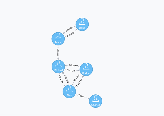
Strongly Connected Components algorithm examples

The following will create a sample graph:

CREATE (nAlice:User {name:'Alice'})
CREATE (nBridget:User {name:'Bridget'})
CREATE (nCharles:User {name:'Charles'})
CREATE (nDoug:User {name:'Doug'})
CREATE (nMark:User {name:'Mark'})
CREATE (nMichael:User {name:'Michael'})

CREATE (nAlice)-[:FOLLOW]->(nBridget)
CREATE (nAlice)-[:FOLLOW]->(nCharles)
CREATE (nMark)-[:FOLLOW]->(nDoug)
CREATE (nMark)-[:FOLLOW]->(nMichael)
CREATE (nBridget)-[:FOLLOW]->(nMichael)
CREATE (nDoug)-[:FOLLOW]->(nMark)
CREATE (nMichael)-[:FOLLOW]->(nAlice)
CREATE (nAlice)-[:FOLLOW]->(nMichael)
CREATE (nBridget)-[:FOLLOW]->(nAlice)
CREATE (nMichael)-[:FOLLOW]->(nBridget);

The following will project and store a named graph:

MATCH (source:User)-[r:FOLLOW]->(target:User)
RETURN gds.graph.project(
  'graph',
  source,
  target
)

Memory Estimation

First off, we will estimate the cost of running the algorithm using the estimate procedure. This can be done with any execution mode. We will use the write mode in this example. Estimating the algorithm is useful to understand the memory impact that running the algorithm on your graph will have. When you later actually run the algorithm in one of the execution modes the system will perform an estimation. If the estimation shows that there is a very high probability of the execution going over its memory limitations, the execution is prohibited. To read more about this, see Automatic estimation and execution blocking.

For more details on estimate in general, see Memory Estimation.

The following will estimate the memory requirements for running the algorithm:

CALL gds.scc.write.estimate('graph', { writeProperty: 'componentId' })
YIELD nodeCount, relationshipCount, bytesMin, bytesMax, requiredMemory

Table 13. Results
nodeCount	relationshipCount	bytesMin	bytesMax	requiredMemory
6	10	33332	33332	"32 KiB"

Stream

In the stream execution mode, the algorithm returns the component for each node. This allows us to inspect the results directly or post-process them in Cypher without any side effects.

For more details on the stream mode in general, see Stream.

The following will run the algorithm and stream back results:

CALL gds.scc.stream('graph', {})
YIELD nodeId, componentId
RETURN gds.util.asNode(nodeId).name AS Name, componentId AS Component
ORDER BY Component, Name DESC

Table 14. Results
Name	Component
`"Michael"`	`0`
`"Bridget"`	`0`
`"Alice"`	`0`
`"Charles"`	`3`
`"Mark"`	`4`
`"Doug"`	`4`

We have 3 strongly connected components in our sample graph.

The first, and biggest, component has members Alice, Bridget, and Michael, while the second biggest component has Doug and Mark. Charles ends up in his own component because there isn’t an outgoing relationship from that node to any of the others.

Stats

In the stats execution mode, the algorithm returns a single row containing a summary of the algorithm result. This execution mode does not have any side effects. It can be useful for evaluating algorithm performance by inspecting the computeMillis return item. In the examples below we will omit returning the timings. The full signature of the procedure can be found in the syntax section.

For more details on the stats mode in general, see Stats.

The following will run the algorithm and returns the result in form of statistical and measurement values

CALL gds.scc.stats('graph')
YIELD componentCount

Table 15. Results
componentCount
3

Mutate

The mutate execution mode extends the stats mode with an important side effect: updating the named graph with a new node property containing the component for that node. The name of the new property is specified using the mandatory configuration parameter mutateProperty. The result is a single summary row, similar to stats, but with some additional metrics. The mutate mode is especially useful when multiple algorithms are used in conjunction.

For more details on the mutate mode in general, see Mutate.

The following will run the algorithm and store the results in graph:

CALL gds.scc.mutate('graph', { mutateProperty: 'componentId'})
YIELD componentCount

Table 16. Results
componentCount
3

Write

The write execution mode extends the stats mode with an important side effect: writing the component for each node as a property to the Neo4j database. The name of the new property is specified using the mandatory configuration parameter writeProperty. The result is a single summary row, similar to stats, but with some additional metrics. The write mode enables directly persisting the results to the database.

For more details on the write mode in general, see Write.